NicheSphere tutorial — Myocardial Infarction (Visium)

NicheSphere is an sc-verse compatible Python library for identifying differentially co-localised cellular niches and the biological processes driving their interactions, based on cell type pair co-localization probabilities across conditions.

Co-localization probabilities can be derived from:

• Deconvoluted Visium / PIC-seq data — probability of finding each cell type in each spot / multiplet

• Single-cell resolved spatial data (MERFISH, CODEX, …) — counting cell boundary overlaps or radius-based neighborhoods per cell type pair

NicheSphere also supports localized process-based differential cell-cell communication analysis using Ligand-Receptor (LR) pair expression data from tools such as LIANA and CrossTalkeR.

In this tutorial we apply NicheSphere to the Myocardial Infarction (MI) Visium atlas from Kuppe et al., 2022, to identify cellular niches and communication changes between myogenic and ischemic heart tissue. We will:

1. Load and inspect the data

2. Compute cell type co-localization probabilities from Visium deconvolution results

3. Test differential co-localization between conditions and build a co-localization network

4. Detect niches and compute niche statistics

5. Load communication data and test localized process-based differential communication

6. Visualize differential communication networks and Sankey diagrams

1. Setup

import anndata as ad

import pandas as pd
import numpy as np
import scipy
import seaborn as sns
import matplotlib.pyplot as plt
import matplotlib.colors as mcolors
import networkx as nx
import warnings
import scanpy as sc
import mudata as md
from community_layout.layout_class import CommunityLayout

warnings.filterwarnings("ignore")

import nichesphere

COMMUNITY LAYOUT: Datashader not found, edge bundling not available

Download data

All data files for this tutorial are available on Zenodo.

Please open a Terminal (or Command Line) in the NicheSphere root folder if you cloned the repo from Github and run the following command to download and extract the dataset:

wget https://zenodo.org/records/21806024/files/data.zip && unzip data.zip && rm data.zip

This will download data.zip, extract its contents into the NicheSphere/data/ folder, and automatically remove the zip archive when finished.

2. Data

We use a subset of the MI atlas with 23 samples (samples with fewer than 1500 cells in the snRNA-seq data were excluded).

Our data is stored in a mudata object containing data from two modalities: snRNA-seq data mudata['sc'] and Visium 10x data mudata['visium'].

mudata['sc'] and mudata['visium'] are like two anndata objects

mudata = md.read('../../data/MIvisium/main_tutorial/2306_HMI_allmodalities.h5mu')
mudata

MuData object with n_obs × n_vars = 76798 × 39120
  2 modalities
    sc:     48547 × 27416
      obs:  'orig_ident', 'nCount_RNA', 'nFeature_RNA', 'percent_mt', 'doublet_score', 'doublet', 'dissociation_s1', 'opt_clust', 'patient', 'batch', 'opt_clust_integrated', 'cell_type', 'ident', 'nFeaturess_RNA', 'cell_subtype2', 'patient_region_id', 'sampleType'
      var:  'n_counts'
      obsm: 'X_harmony', 'X_pca', 'X_umap_harmony'
    visium: 28251 × 11704
      obs:  'n_counts', 'n_genes', 'percent.mt', 'Adipocyte', 'Cardiomyocyte', 'Endothelial', 'Fibroblast', 'Lymphoid', 'Mast', 'Myeloid', 'Neuronal', 'Pericyte', 'Cycling.cells', 'vSMCs', 'cell_type_original', 'assay_ontology_term_id', 'cell_type_ontology_term_id', 'development_stage_ontology_term_id', 'disease_ontology_term_id', 'ethnicity_ontology_term_id', 'is_primary_data', 'organism_ontology_term_id', 'sex_ontology_term_id', 'tissue_ontology_term_id', 'patient_region_id', 'orig_ident', 'batch'
      var:  'features'
      obsm: 'X_pca', 'X_spatial', 'X_umap'

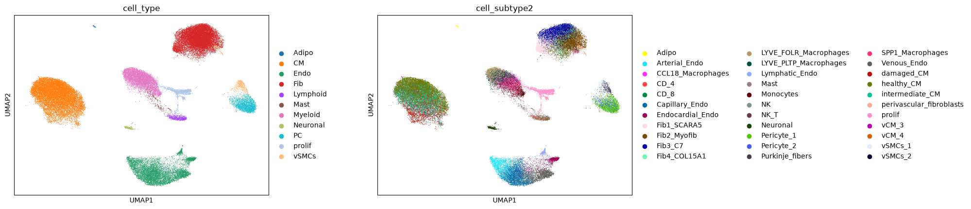
In our snRNA-seq data, we have 11 cell types, stored in mudata['sc'].obs['cell_type'] and 33 cell subtypes, stored in mudata['sc'].obs['cell_subtype2']

mudata['sc'].obsm['umap'] = mudata['sc'].obsm['X_umap_harmony']
sc.pl.umap(mudata['sc'], color=['cell_type', 'cell_subtype2'], wspace=0.3)

3. Co-localization

Cell type proportions per spot

We deconvoluted cell subtypes in the Visium slices using MOSCOT (Klein et al., 2025), obtaining per-cell probabilities of being in each spot. nichesphere.tl.get_spot_ct_props sums these probabilities per cell type to give cell type proportion matrices per spot.

Below we show this for two example samples. The sample the cells or spots come from is indicated in the patient_region_id column in the obs slot of our snRNA-seq and Visium data: mudata['sc'].obs.patient_region_id and mudata['visium'].obs.patient_region_id

The full table for all 23 samples is available directly from Zenodo.

CTprops = pd.DataFrame()
for smpl in ['control_P1', 'GT_IZ_P9']:
    t = pd.read_csv(f'../../data/MIvisium/main_tutorial/cell_probs_{smpl}.csv', index_col=0)

    adata_sc = mudata['sc'][mudata['sc'].obs.patient_region_id == smpl]
    # Keep only cell types with more than 2 cells in this sample
    adata_sc = adata_sc[[
        c in adata_sc.obs.cell_subtype2.value_counts().index[
            adata_sc.obs.cell_subtype2.value_counts() > 2
        ] for c in adata_sc.obs.cell_subtype2
    ]]

    props = nichesphere.tl.get_spot_ct_props(
        spot_cell_props=t,
        sc_ct=adata_sc.obs.cell_subtype2
    )
    CTprops = pd.concat([CTprops, props])

Load the full cell type proportions table (all 23 samples) from Zenodo:

CTprops = pd.read_csv('../../data/MIvisium/main_tutorial/CTprops.csv', index_col=0)
## Subset as we just use 9 samples for this tutorial
CTprops=CTprops.loc[mudata['visium'].obs.index]
CTprops.head()

	Fib1_SCARA5	damaged_CM	Capillary_Endo	LYVE_FOLR_Macrophages	Fib3_C7	healthy_CM	Fib2_Myofib	Endocardial_Endo	Arterial_Endo	Neuronal	...	CCL18_Macrophages	perivascular_fibroblasts	CD_4	vSMCs_2	Lymphatic_Endo	NK	CD_8	Purkinje_fibers	Adipo	NK_T
AAACAAGTATCTCCCA-1-0-0-0-0-0-0-0-0-0-0-0-0-0-0-0-0-0-0-0-0-0-0	0.0	0.000000	0.0	0.0	0.000000	1.000000	0.0	0.0	1.249070e-32	0.0	...	0.0	0.0	0.000000	0.0	0.0	0.0	0.0	0.0	NaN	0.0
AAACACCAATAACTGC-1-0-0-0-0-0-0-0-0-0-0-0-0-0-0-0-0-0-0-0-0-0-0	0.0	0.000000	0.0	0.0	0.000000	0.000000	0.0	0.0	0.000000e+00	0.0	...	0.0	0.0	0.341564	0.0	0.0	0.0	0.0	0.0	NaN	0.0
AAACAGCTTTCAGAAG-1-0-0-0-0-0-0-0-0-0-0-0-0-0-0-0-0-0-0-0-0-0-0	0.0	0.000000	0.0	0.0	0.358745	0.282511	0.0	0.0	0.000000e+00	0.0	...	0.0	0.0	0.000000	0.0	0.0	0.0	0.0	0.0	NaN	0.0
AAACAGGGTCTATATT-1-0-0-0-0-0-0-0-0-0-0-0-0-0-0-0-0-0-0-0-0-0-0	0.0	0.328716	0.0	0.0	0.000000	0.335562	0.0	0.0	0.000000e+00	0.0	...	0.0	0.0	0.000000	0.0	0.0	0.0	0.0	0.0	NaN	0.0
AAACCGGGTAGGTACC-1-0-0-0-0-0-0-0-0-0-0-0-0-0-0-0-0-0-0-0-0-0-0	0.0	0.000000	0.0	0.0	0.994955	0.005045	0.0	0.0	0.000000e+00	0.0	...	0.0	0.0	0.000000	0.0	0.0	0.0	0.0	0.0	NaN	0.0

5 rows × 33 columns

Inspecting deconvolution results

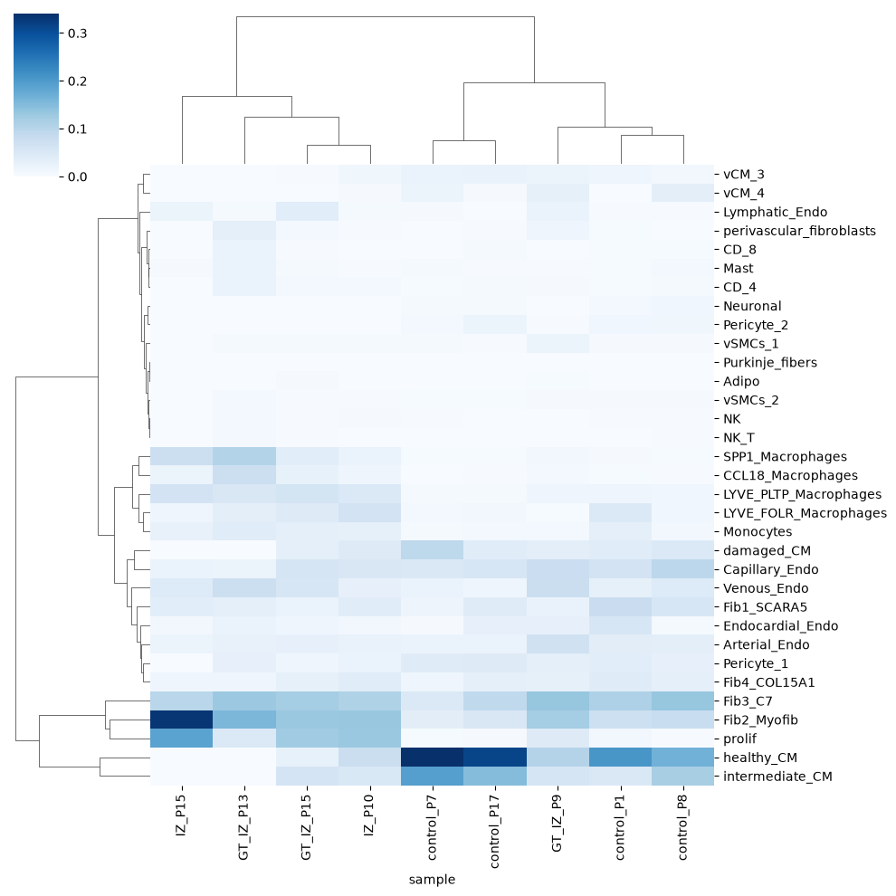
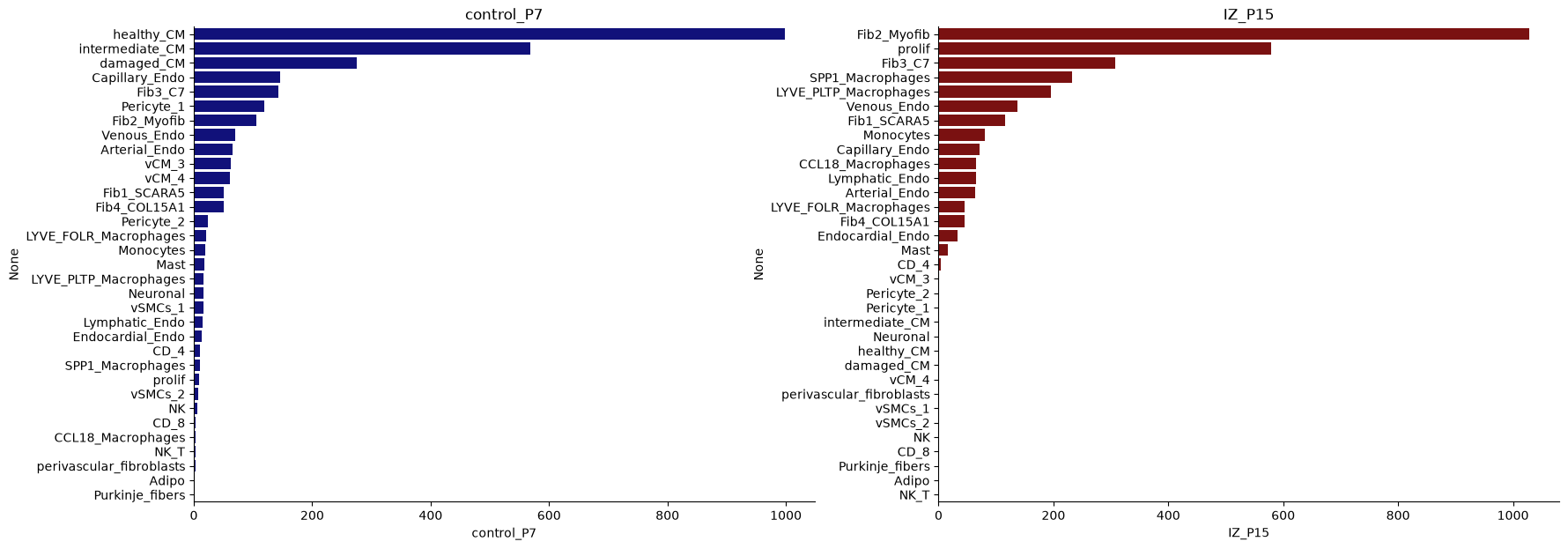
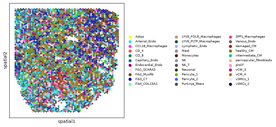
We can check cell type proportions per sample with a clustermap or barplots, and visualize the dominant cell type per spot in a Visium slice.

spotSamples = mudata['visium'].obs.patient_region_id

CTprops_sample = CTprops.loc[spotSamples.index].copy()
CTprops_sample['sample'] = spotSamples.values
sns.clustermap(
    CTprops_sample.groupby('sample').sum().T /
    CTprops_sample.groupby('sample').sum().sum(axis=1),
    cmap='Blues', method='ward'
)

<seaborn.matrix.ClusterGrid at 0x1554458d9370>

t1 = pd.DataFrame(CTprops[spotSamples == 'control_P7'].sum(), columns=['control_P7'])
t2 = pd.DataFrame(CTprops[spotSamples == 'IZ_P15'].sum(), columns=['IZ_P15'])

fig, axes = plt.subplots(1, 2, figsize=(20, 7))
sns.set_style(rc={'axes.facecolor': 'white'})

sns.barplot(ax=axes[0], y=t1.sort_values('control_P7', ascending=False).index,
            x='control_P7', data=t1.sort_values('control_P7', ascending=False), color='darkblue')
axes[0].set_title('control_P7')

sns.barplot(ax=axes[1], y=t2.sort_values('IZ_P15', ascending=False).index,
            x='IZ_P15', data=t2.sort_values('IZ_P15', ascending=False), color='darkred')
axes[1].set_title('IZ_P15')
sns.despine()

We can also color each Visium spot by the cell type with the highest proportion using nichesphere.coloc.spatialCTPlot:

mudata['visium'].uns['spatial'] = mudata['visium'].obsm['X_spatial']

idPat = 'GT_IZ_P9'
nichesphere.coloc.spatialCTPlot(
    adata=mudata['visium'][mudata['visium'].obs.patient_region_id == idPat].copy(),
    CTprobs=CTprops.loc[spotSamples.index[spotSamples == idPat]],
    cell_types=mudata['sc'].obs.cell_subtype2,
    spot_size=0.015,
    legend_fontsize=7
)

WARNING: saving figure to file figures/showtest.pdf

Co-localization probabilities

nichesphere.coloc.getColocProbs computes concatenated co-localization matrices (cell type × cell type) per sample based on the probabilities of each cell type per spot. If additional information on the number of cells per spot is available (eg: an estimated number of cells per spot by cell2location), spot weights can be added to the co-localization probabilities calculations via the spotweights parameter.

CTcolocalizationP = nichesphere.coloc.getColocProbs(
    CTprobs=CTprops,
    spotSamples=mudata['visium'].obs.patient_region_id
)

reshapeColoc then pivots these into a cell type pair × sample matrix. Setting complete=1 indicates that both directions of each pair (ct1–ct2 and ct2–ct1) are present in the data.

As a safety check, we sum the co-localization probabilities across all cell pairs per sample. They should sum up to 1 per sample.

If co-localization probabilities do not sum up to 1, it might be worth checking if the given ``CTprobs`` are indeed cell type probabilities per spot (they should also sum up to 1 per spot).

colocPerSample = nichesphere.coloc.reshapeColoc(CTcoloc=CTcolocalizationP, complete=1)
colocPerSample=colocPerSample.fillna(0)
colocPerSample.sum(axis=1)  # should be ~1.0 for every sample

GT_IZ_P13      1.0
GT_IZ_P15      1.0
GT_IZ_P9       1.0
IZ_P10         1.0
IZ_P15         1.0
control_P1     1.0
control_P17    1.0
control_P7     1.0
control_P8     1.0
dtype: float64

colocPerSample.head()

	Fib1_SCARA5-Fib1_SCARA5	Fib1_SCARA5-damaged_CM	Fib1_SCARA5-Capillary_Endo	Fib1_SCARA5-LYVE_FOLR_Macrophages	Fib1_SCARA5-Fib3_C7	Fib1_SCARA5-healthy_CM	Fib1_SCARA5-Fib2_Myofib	Fib1_SCARA5-Endocardial_Endo	Fib1_SCARA5-Arterial_Endo	Fib1_SCARA5-Neuronal	...	NK_T-CCL18_Macrophages	NK_T-perivascular_fibroblasts	NK_T-CD_4	NK_T-vSMCs_2	NK_T-Lymphatic_Endo	NK_T-NK	NK_T-CD_8	NK_T-Purkinje_fibers	NK_T-Adipo	NK_T-NK_T
GT_IZ_P13	0.018084	0.000000	0.000154	3.540328e-04	0.003069	0.000000e+00	0.002831	4.390572e-04	0.000276	0.0	...	8.345726e-05	1.007656e-05	0.00026	0.0	0.000000e+00	0.000000	3.963644e-04	0.0	0.0	0.004869
GT_IZ_P15	0.020017	0.000040	0.000107	1.413835e-05	0.000772	4.690843e-16	0.000702	6.130994e-09	0.000152	0.0	...	0.000000e+00	7.448928e-30	0.00000	0.0	3.143464e-46	0.000000	3.756373e-28	0.0	0.0	0.001477
GT_IZ_P9	0.019715	0.000200	0.000250	3.609267e-33	0.000643	3.859817e-04	0.000741	2.134773e-04	0.000366	0.0	...	0.000000e+00	0.000000e+00	0.00000	0.0	0.000000e+00	0.000000	0.000000e+00	0.0	0.0	0.000000
IZ_P10	0.030229	0.000096	0.000610	3.347724e-04	0.002416	1.363541e-05	0.001721	1.966849e-04	0.000138	0.0	...	6.626314e-36	0.000000e+00	0.00000	0.0	0.000000e+00	0.000024	0.000000e+00	0.0	0.0	0.000857
IZ_P15	0.030351	0.000000	0.000027	1.859005e-04	0.001200	0.000000e+00	0.003112	7.228002e-05	0.000062	0.0	...	0.000000e+00	0.000000e+00	0.00000	0.0	0.000000e+00	0.000000	0.000000e+00	0.0	0.0	0.000000

5 rows × 1089 columns

Sample–condition mapping

Condition is encoded in sample name abbreviations: RZ = Remote zone, BZ = Border zone, FZ = Fibrotic zone, IZ = Ischemic zone. Everything else is myogenic (healthy).

sampleTypesDF = pd.DataFrame(colocPerSample.index, columns=['sample'])
sampleTypesDF['sampleType'] = 'myogenic'
for abbrev, label in [('RZ', 'remote'), ('BZ', 'border'), ('FZ', 'fibrotic'), ('IZ', 'ischemic')]:
    sampleTypesDF.loc[sampleTypesDF['sample'].str.contains(abbrev), 'sampleType'] = label
sampleTypesDF.head()

	sample	sampleType
0	GT_IZ_P13	ischemic
1	GT_IZ_P15	ischemic
2	GT_IZ_P9	ischemic
3	IZ_P10	ischemic
4	IZ_P15	ischemic

We also build the list of same-cell-type pairs (e.g. CM-CM), which will be excluded from differential testing:

cell_types = CTprops.columns
oneCTints = cell_types + '-' + cell_types

4. Differential co-localization

We test differential co-localization between myogenic and ischemic samples using Wilcoxon rank-sum tests (one test per cell type pair):

• H₀: The median difference in co-localization probability between myogenic and ischemic samples is zero.

• H₁: The median difference is non-zero.

myo_iscDF = nichesphere.coloc.diffColoc_test(
    coloc_pair_sample=colocPerSample,
    sampleTypes=sampleTypesDF,
    exp_condition='ischemic',
    ctrl_condition='myogenic'
)
myo_iscDF.head()

	pairs	statistic	p-value
pairs
Fib1_SCARA5-Fib1_SCARA5	Fib1_SCARA5-Fib1_SCARA5	0.489898	0.624206
Fib1_SCARA5-damaged_CM	Fib1_SCARA5-damaged_CM	-2.44949	0.014306
Fib1_SCARA5-Capillary_Endo	Fib1_SCARA5-Capillary_Endo	-2.204541	0.027486
Fib1_SCARA5-LYVE_FOLR_Macrophages	Fib1_SCARA5-LYVE_FOLR_Macrophages	-0.489898	0.624206
Fib1_SCARA5-Fib3_C7	Fib1_SCARA5-Fib3_C7	-2.44949	0.014306

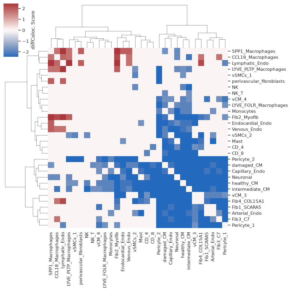
nichesphere.tl.pval_filtered_HMdf reshapes the test results into a cell type × cell type heatmap matrix, setting non-significant scores (p > p) to 0. We then remove proliferating cells (hard to interpret as a single cell type) and any cell types with no significant co-localization changes.

myo_isc_HM = nichesphere.tl.pval_filtered_HMdf(
    testDF=myo_iscDF,
    oneCTinteractions=oneCTints,
    p=0.1,
    cell_types=cell_types
)

# Remove proliferating cells and rows/columns with all-zero scores
myo_isc_HM = myo_isc_HM.loc[
    ~myo_isc_HM.columns.str.contains('prolif'),
    ~myo_isc_HM.index.str.contains('prolif')
]
myo_isc_HM = myo_isc_HM.loc[myo_isc_HM.sum() != 0, myo_isc_HM.sum() != 0]

sns.set(font_scale=1)
sns.clustermap(myo_isc_HM, cmap='vlag', center=0, method='ward',
               cbar_kws={'label': 'diffColoc. Score'})

<seaborn.matrix.ClusterGrid at 0x15543f5f8800>

5. Differential co-localization network and niche detection

Adjacency matrix

We build an adjacency matrix from Euclidean distances between each cell type’s differential co-localization profile. Cell types with no significant differential co-localization receive a weight of 0.

HMdist = pd.DataFrame(
    scipy.spatial.distance.squareform(scipy.spatial.distance.pdist(myo_isc_HM)),
    columns=myo_isc_HM.columns, index=myo_isc_HM.index
)
HMsimm = 1 - HMdist / HMdist.max().max()
HMsimm[myo_isc_HM == 0] = 0

Initial network

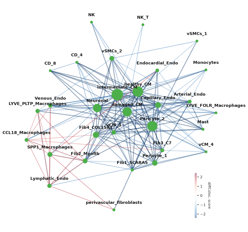
We first plot the network with all nodes in a single placeholder group to get a visual overview before community detection.

colocNW parameters:

• nodeSize: size of nodes by network statistic — 'betweeness', 'pagerank', or None (uniform)

• alpha: edge transparency (0–1)

• edge_scale: edge width multiplier

niches_dict = {'1_': list(myo_isc_HM.index)}
clist = ['#4daf4a']

plt.rcParams['axes.facecolor'] = 'None'
nichesphere.coloc.colocNW(
    x_diff=myo_isc_HM,
    adj=HMsimm,
    cell_group=niches_dict,
    clist=clist,
    nodeSize='betweeness',
    lab_spacing=9,
    alpha=0.4,
    fsize=(12, 12)
)

<networkx.classes.graph.Graph at 0x155441033e60>

Niche detection

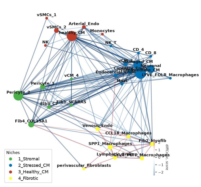
We detect communities (niches) using Louvain clustering on the unsigned adjacency network, then use CommunityLayout to position nodes so that niches are spatially grouped. CommunityLayout is compatible with any NetworkX community detection function, specified via community_algorithm and community_kwargs.

gCol_unsigned = nx.from_pandas_adjacency(HMsimm, create_using=nx.Graph)

cl = CommunityLayout(
    gCol_unsigned,
    community_compression=0.4,
    layout_algorithm=nx.spring_layout,
    layout_kwargs={"k": 75, "iterations": 1000},
    community_algorithm=nx.algorithms.community.louvain_communities,
    community_kwargs={"resolution": 1.1, "seed": 12, "weight": "weight"}
)

d = {i: list(v) for i, v in enumerate(cl.communities())}
print(pd.DataFrame.from_dict(d, orient='index').T.to_string(index=False))

Building meta-graph
Metagraph is a Graph with 4 nodes and 6 edges

100%|██████████| 4/4 [00:00<00:00, 342.11it/s]

           0                     1             2                        3
  Pericyte_1                  Mast            NK              Venous_Endo
Fib4_COL15A1       intermediate_CM Arterial_Endo           Lymphatic_Endo
       vCM_4        Capillary_Endo       vSMCs_1         SPP1_Macrophages
  Pericyte_2                 vCM_3       vSMCs_2        CCL18_Macrophages
 Fib1_SCARA5                  CD_8    healthy_CM    LYVE_PLTP_Macrophages
     Fib3_C7              Neuronal     Monocytes              Fib2_Myofib
        None      Endocardial_Endo          None perivascular_fibroblasts
        None                  NK_T          None                     None
        None LYVE_FOLR_Macrophages          None                     None
        None                  CD_4          None                     None
        None            damaged_CM          None                     None

niche_names = ['1_Stromal', '2_Stressed_CM', '3_Healthy_CM', '4_Fibrotic']
niches_dict = dict(zip(niche_names, list(d.values())))

clist = ['#4daf4a', '#0072B5', '#BC3C29', '#ffff33']
niche_cols = pd.Series(clist, index=list(niches_dict.keys()))
niches_df = nichesphere.tl.cells_niche_colors(
    CTs=CTprops.columns, niche_colors=niche_cols, niche_dict=niches_dict
)
niches_df.head()

	cell	niche	color
cell
Fib1_SCARA5	Fib1_SCARA5	1_Stromal	#4daf4a
damaged_CM	damaged_CM	2_Stressed_CM	#0072B5
Capillary_Endo	Capillary_Endo	2_Stressed_CM	#0072B5
LYVE_FOLR_Macrophages	LYVE_FOLR_Macrophages	2_Stressed_CM	#0072B5
Fib3_C7	Fib3_C7	1_Stromal	#4daf4a

Final network plot

We pass the community-aware node positions via pos and set layout=None:

pos = cl.full_positions

plt.rcParams['axes.facecolor'] = 'None'
gCol = nichesphere.coloc.colocNW(
    x_diff=myo_isc_HM,
    adj=HMsimm,
    cell_group=niches_dict,
    clist=clist,
    nodeSize='betweeness',
    layout=None,
    lab_spacing=0.05,
    thr=1,
    alpha=0.4,
    fsize=(10, 10),
    pos=pos,
    edge_scale=1,
    legend_ax=[0.7, 0.05, 0.15, 0.2]
)

legend_elements = [
    plt.Line2D([0], [0], marker='o', color='w', markerfacecolor=clist[i],
               lw=4, label=list(niches_dict.keys())[i], ms=10)
    for i in range(len(niches_dict))
]
plt.gca().add_artist(
    plt.legend(handles=legend_elements, loc='lower left', fontsize=13,
               title='Niches', alignment='left')
)
# plt.savefig('diffColocNW.pdf')

<matplotlib.legend.Legend at 0x155445cfb350>

We save the network and node positions for reuse in the communication section:

#nx.write_graphml_lxml(gCol, 'data/colocNW_MIvisium_louvain.graphml')
#np.save('data/colocNW_pos.npy', pos)

We also save the niche–cell type correspondence and co-localization filter tables, needed for differential communication:

#niches_df.to_csv('data/niches_df_MIvisium_louvain.csv')

pairCatDFdir = nichesphere.tl.get_pairCatDFdir(niches_df)
#pairCatDFdir.to_csv('data/pairCatDFdir_MIvisium_louvain.csv')

# Flag differentially co-localized cell pairs (filter=1 → will be tested in comm analysis)
pairCatDF_filter = [
    (pairCatDFdir.cell_pairs.str.split('->')[i][0] in HMsimm.index) and
    (pairCatDFdir.cell_pairs.str.split('->')[i][1] in HMsimm.index)
    for i in pairCatDFdir.index
]
pairCatDFdir_filt = pairCatDFdir[pairCatDF_filter]
oneCTints_filt = oneCTints[[i.split('-')[0] in HMsimm.index for i in oneCTints]]

colocFilt = nichesphere.tl.getColocFilter(
    pairCatDF=pairCatDFdir_filt,
    adj=HMsimm,
    oneCTints=oneCTints_filt.str.replace('-', '->')
)
#colocFilt.to_csv('data/colocFilt_MIvisium_louvain.csv')
colocFilt.head()

	filter
cell_pairs
Fib1_SCARA5->Fib1_SCARA5	1.0
Fib1_SCARA5->damaged_CM	1.0
Fib1_SCARA5->Capillary_Endo	1.0
Fib1_SCARA5->LYVE_FOLR_Macrophages	0.0
Fib1_SCARA5->Fib3_C7	1.0

We also assign niche/community properties to the network object for downstream use:

nichesphere.tl.assign_properties(
    gCol,
    communities=cl.communities(),
    colors=clist,
    pos=pos,
    simmilarity_weights=True,
    node_coord_sf=100,
    g_unsigned=gCol_unsigned
)

Interactive network

The gravis library enables an interactive D3-based network visualization where node sizes, edge widths, and label sizes can be adjusted in the browser. One can also move the nodes around to avoid overlaps.

Note: gravis may require downgrading setuptools: pip install --force-reinstall -U "setuptools<82.0.0"

import gravis as gv
gv.d3(gCol, edge_size_data_source='weight_abs', zoom_factor=0.35, layout_algorithm_active=False)

Details for selected element

General

App state

Reset

Display mode

Enter full screen

Export

SVG PNG JPG

Data selection

Graph

Node label text

Edge label text

Node size

Normalize

Minimum

Maximum

Edge size

Normalize

Minimum

Maximum

Nodes

Visibility

Show nodes

Size

Scaling factor

Position

Release fixed nodes

Drag behavior

Fix node position

Hover behavior

Show neighborhood

Show tooltips (if provided)

Node images

Visibility

Show node images

Size

Scaling factor

Node labels

Visibility

Show node labels

Show borders

Size

Scaling factor

Rotation

Angle

Edges

Visibility

Show edges

Size

Scaling factor

Form

Curvature

Hover behavior

Show tooltips (if provided)

Edge labels

Visibility

Show edge labels

Show borders

Size

Scaling factor

Rotation

Angle

Layout algorithm

Simulation

Active

Many-body force

On

Strength

Theta

Use minimum distance

Min

Use maximum distance

Max

Links force

On

Distance

Strength

Collision force

On

Radius

Strength

x-positioning force

On

Strength

y-positioning force

On

Strength

Centering force

On

6. Network statistics

nichesphere.tl.compute_network_stats computes betweenness centrality, PageRank, and signed degree centrality (split into positive and negative edges) for the co-localization network. plot_top_stats visualises the top nodes for each metric.

nw_stats = nichesphere.tl.compute_network_stats(gCol)
nw_stats.head()

	betweenness	pagerank	degree_positive	degree_negative
Fib1_SCARA5	-24.303800	-1.706905	0.000000	0.413793
damaged_CM	-29.868265	-2.560918	0.000000	0.758621
Capillary_Endo	-28.048485	-2.250336	0.000000	0.620690
LYVE_FOLR_Macrophages	0.000000	-0.726972	0.000000	0.206897
Fib3_C7	-24.028574	-0.499136	0.034483	0.413793

sns.set(font_scale=2)
plt.rcParams['axes.facecolor'] = 'None'
f=nichesphere.tl.plot_top_stats(nw_stats, top_n=5)
# f.savefig('diffColocNW_stats.pdf', bbox_inches='tight')

7. Niche statistics

The nichesphere.niche_stats module provides tools to assess the internal cohesion of each niche relative to its cross-niche connections, using the signed edge weight distribution.

community_edge_stats_df returns a summary table of positive/negative edge counts and weights per niche:

vc_map_named = {node: niche for niche, members in niches_dict.items() for node in members}

edge_stats = nichesphere.niche_stats.community_edge_stats_df(gCol, vc_map_named)
edge_stats

	internal_pos_count	internal_pos_weight	internal_neg_count	internal_neg_weight	external_pos_count	external_pos_weight	external_neg_count	external_neg_weight
community
1_Stromal	0	0.000000	14	32.578214	3	5.633826	54	122.719436
2_Stressed_CM	0	0.000000	36	80.833162	1	1.959592	69	155.175175
3_Healthy_CM	0	0.000000	9	17.758801	0	0.000000	41	93.570508
4_Fibrotic	15	30.251198	0	0.000000	4	7.593418	26	55.480943

plot_internal_external_boxplots visualises the signed internal vs external edge weight distributions per niche. Niches where internal weights are higher than external weights are more cohesively co-localised internally than across niches.

sns.set(font_scale=1)
plt.rcParams['axes.facecolor'] = 'None'
nichesphere.niche_stats.plot_internal_external_boxplots(gCol, vc_map_named)
# plt.savefig('niche_internal_external_weights.pdf', bbox_inches='tight')

<Axes: title={'center': 'Internal vs external edge weight distributions by niche'}, xlabel='niche', ylabel='edge weight'>

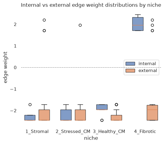
A Wilcoxon rank-sum test can confirm whether internal and external weight distributions are significantly different per niche:

signed = nichesphere.niche_stats.community_signed_weight_distributions(gCol, vc_map_named)
communities = list(signed.keys())

pairwise_stats = nichesphere.niche_stats.pairwise_ranksums_int_ext(
    data_int=[signed[c]['internal'] for c in communities],
    data_ext=[signed[c]['external'] for c in communities],
    communities=communities
)
pairwise_stats

	niche	statistic	p_value	p_value_corrected
0	1_Stromal	-0.498588	0.618069	0.824093
1	2_Stressed_CM	-0.026684	0.978711	0.978711
2	3_Healthy_CM	2.487302	0.012872	0.025743
3	4_Fibrotic	4.851550	0.000001	0.000005

8. Niche visualization in Visium slices

nichesphere.coloc.spatialNichePlot colors each spot by the niche of the cell type with the highest proportion.

fig, axes = plt.subplots(2, 3, figsize=(21, 14))
plt.close(fig)

for idu, smpl in enumerate(sampleTypesDF['sample'][sampleTypesDF['sampleType'] == 'myogenic'][:3]):
    nichesphere.coloc.spatialNichePlot(
        adata=mudata['visium'][mudata['visium'].obs.patient_region_id == smpl].copy(),
        CTprobs=CTprops.loc[spotSamples.index[spotSamples == smpl]],
        niche_dict=niches_dict,
        spot_size=0.015,
        niche_colors=niche_cols,
        legend_fontsize=7,
        #save_name=f'_{smpl}.pdf',
        ax=axes[0][idu]
    )

for idu, smpl in enumerate(sampleTypesDF['sample'][sampleTypesDF['sampleType'] == 'ischemic'][:3]):
    nichesphere.coloc.spatialNichePlot(
        adata=mudata['visium'][mudata['visium'].obs.patient_region_id == smpl].copy(),
        CTprobs=CTprops.loc[spotSamples.index[spotSamples == smpl]],
        niche_dict=niches_dict,
        spot_size=0.015,
        niche_colors=niche_cols,
        legend_fontsize=7,
        #save_name=f'_{smpl}.pdf',
        ax=axes[1][idu]
    )

fig.tight_layout()
fig

WARNING: saving figure to file figures/showtest.pdf

<Figure size 640x480 with 0 Axes>

WARNING: saving figure to file figures/showtest.pdf

<Figure size 640x480 with 0 Axes>

WARNING: saving figure to file figures/showtest.pdf

<Figure size 640x480 with 0 Axes>

WARNING: saving figure to file figures/showtest.pdf

<Figure size 640x480 with 0 Axes>

WARNING: saving figure to file figures/showtest.pdf

<Figure size 640x480 with 0 Axes>

WARNING: saving figure to file figures/showtest.pdf

<Figure size 640x480 with 0 Axes>

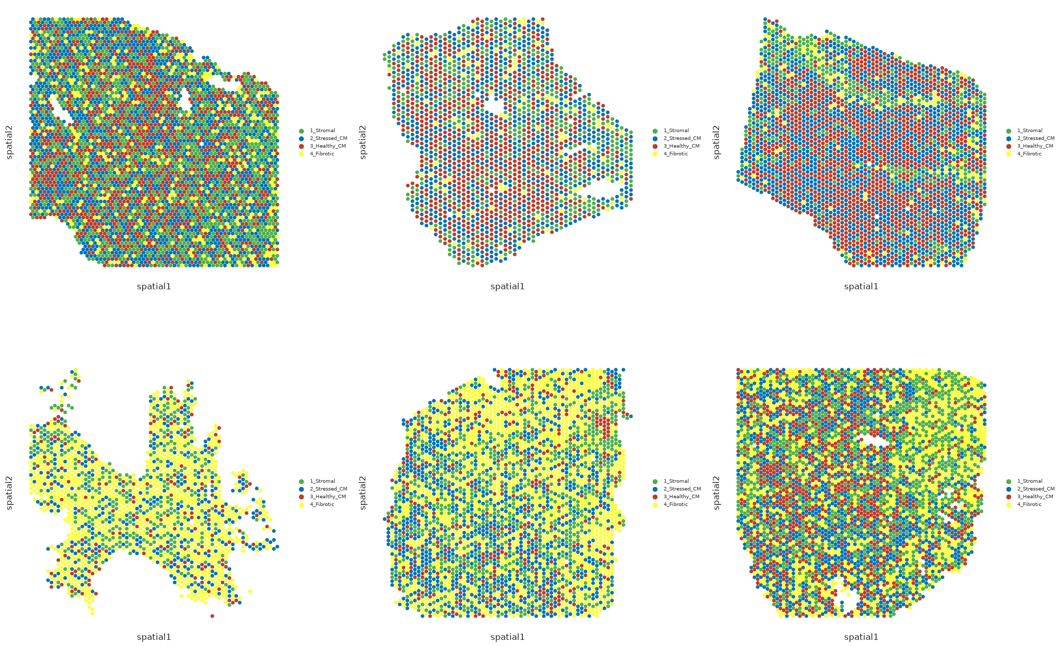
9. Communication data

To compute localized differential communication, we need per-condition LR interaction scores. We derive these by running LIANA on the scRNA-seq data per condition, then converting the results to pyCrossTalkeR format for the differential analysis.

Prepare scRNA-seq data for LIANA

LIANA requires raw counts. The mudata['sc'] object contains the processed scRNA-seq data; we build a lightweight raw-count AnnData from its counts layer, sharing obs and var without copying the full object.

adata_sc_raw=sc.read_h5ad('../../data/MIvisium/main_tutorial/snRNAseq_cellsWithSubtype_sampleType.h5ad')

## Subset for the samples we use
adata_sc_raw=adata_sc_raw[mudata['sc'].obs.index]

import anndata as ad
import liana as li
import os
from pycrosstalker import tools as cttl

adata_sc_raw.raw = adata_sc_raw

Run LIANA per condition

We run LIANA’s CellPhoneDB method on the scRNA-seq data of each condition separately, using cell_subtype2 as the grouping variable. We use the human consensus resource (humanconsensus); adjust resource_name if your data is from another species.

Note: This step can take several minutes per condition. The precomputed tables are available on Zenodo if you prefer to skip it (see below).

adata_sc_raw.uns['liana'] = {}

conditions = sampleTypesDF['sampleType'].unique()
for cond in conditions:
    samples_in_cond = sampleTypesDF.loc[sampleTypesDF['sampleType'] == cond, 'sample']
    adata_cond = adata_sc_raw[adata_sc_raw.obs['patient_region_id'].isin(samples_in_cond)]

    lr = li.method.cellphonedb(
        adata_cond,
        groupby='cell_subtype2',
        expr_prop=0.1,
        verbose=True,
        resource_name='consensus',
        inplace=False
    )
    adata_sc_raw.uns['liana'][cond] = lr

Using resource `consensus`.
Using `.raw`!
Converting to sparse csr matrix!
8587 features of mat are empty, they will be removed.
Make sure that normalized counts are passed!
0.29 of entities in the resource are missing from the data.

Generating ligand-receptor stats for 16776 samples and 1245 features

100%|██████████| 1000/1000 [01:30<00:00, 11.02it/s]
Using resource `consensus`.
Using `.raw`!
Converting to sparse csr matrix!
2340 features of mat are empty, they will be removed.
Make sure that normalized counts are passed!
0.17 of entities in the resource are missing from the data.

Generating ligand-receptor stats for 31771 samples and 1504 features

100%|██████████| 1000/1000 [04:30<00:00,  3.69it/s]

Convert to pyCrossTalkeR and run differential analysis

cttl.utils.from_liana converts the LIANA output into pyCrossTalkeR format. cttl.analise_LR then runs the differential LR analysis between conditions, producing per-condition communication tables and a comparison table (ischemic_x_myogenic).

adata_sc_raw = cttl.utils.from_liana(adata_sc_raw)
adata_sc_raw.uns['pycrosstalker']['details'] = {'filename': 'MIvisium'}

output = 'results/output_ctkr/MIvisium/'
os.makedirs(output, exist_ok=True)

adata_sc_raw = cttl.analise_LR(
    adata_sc_raw,
    out_path=output,
    comparison=[('ischemic', 'myogenic')]
)

Create a Differential Table
Calculating CCI Ranking
Calculating GCI Ranking
Network Analysis Done
Generating h5ad file with Analysed Results

Retrieve communication tables

We retrieve the per-condition LR tables from the pyCrossTalkeR output. nichesphere.tl.processCTKRoutput strips the |L, |R, and |TF suffixes that CrossTalkeR appends to gene names, which can otherwise conflict with downstream matching against the ligand database.

crossTalker_myoComm = adata_sc_raw.uns['pycrosstalker']['path']['myogenic']
crossTalker_iscComm = adata_sc_raw.uns['pycrosstalker']['path']['ischemic']

crossTalker_myoComm = nichesphere.tl.processCTKRoutput(crossTalker_myoComm)
crossTalker_iscComm = nichesphere.tl.processCTKRoutput(crossTalker_iscComm)

# Restrict to cell type pairs present in the co-localization network.
# pairCatDFdir only contains pairs that passed the differential co-localization
# filter; pairs absent from it (e.g. cell types removed during preprocessing)
# would cause a KeyError in lr_ctPairScores_perCat_dir.
valid_pairs = set(pairCatDFdir['cell_pairs'])
crossTalker_myoComm = crossTalker_myoComm[
    (crossTalker_myoComm['source'] + '->' + crossTalker_myoComm['target']).isin(valid_pairs)
]
crossTalker_iscComm = crossTalker_iscComm[
    (crossTalker_iscComm['source'] + '->' + crossTalker_iscComm['target']).isin(valid_pairs)
]

crossTalker_myoComm.head()

	source	target	type_gene_A	type_gene_B	gene_A	gene_B	MeanLR	cellpair	ligpair	recpair	allpair	LRScore
273495	intermediate_CM	healthy_CM	Ligand	Receptor	CALM1	RYR2	147.945694	intermediate_CM@healthy_CM	intermediate_CM/CALM1|L	healthy_CM/RYR2|R	intermediate_CM/CALM1@healthy_CM/RYR2	147.945694
264705	Endocardial_Endo	healthy_CM	Ligand	Receptor	CALM1	RYR2	147.889618	Endocardial_Endo@healthy_CM	Endocardial_Endo/CALM1|L	healthy_CM/RYR2|R	Endocardial_Endo/CALM1@healthy_CM/RYR2	147.889618
272920	healthy_CM	healthy_CM	Ligand	Receptor	CALM1	RYR2	147.882706	healthy_CM@healthy_CM	healthy_CM/CALM1|L	healthy_CM/RYR2|R	healthy_CM/CALM1@healthy_CM/RYR2	147.882706
275547	vCM_4	healthy_CM	Ligand	Receptor	CALM1	RYR2	147.870972	vCM_4@healthy_CM	vCM_4/CALM1|L	healthy_CM/RYR2|R	vCM_4/CALM1@healthy_CM/RYR2	147.870972
288072	intermediate_CM	intermediate_CM	Ligand	Receptor	CALM1	RYR2	147.856003	intermediate_CM@intermediate_CM	intermediate_CM/CALM1|L	intermediate_CM/RYR2|R	intermediate_CM/CALM1@intermediate_CM/RYR2	147.856003

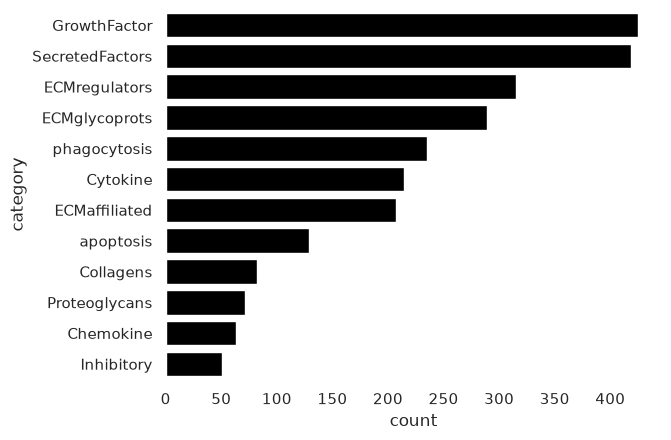
Ligand-process database

We use the NicheSphere database, which classifies ligands according to ECM-related and immune recruitment processes. It is available in the NicheSphere GitHub repository.

import nichesphere.database as db

# Load database
allDBs = nichesphere.load_DB()

sns.barplot(x=allDBs.category.value_counts(), y=allDBs.category.value_counts().index,
            data=pd.DataFrame(allDBs.category.value_counts()), color='black')
sns.despine()

lr_ctPairScores_perCat_dir separates communication scores by biological process, computing the mean LR score per cell type pair per process category. equalizeScoresTables assigns 0 to interactions absent in one condition so both are directly comparable.

myoCTpairScores = nichesphere.comm.lr_ctPairScores_perCat_dir(
    ccommTable=crossTalker_myoComm,
    db=allDBs, dbCatCol='category', dbMatchCol='Ligand',
    ccommMatchCol='gene_A', ccommLRscoresCol='MeanLR',
    oneCTinteractions=oneCTints.str.replace('-', '@'),
    condition='myogenic',
    pairCatDF=pairCatDFdir
)

iscCTpairScores = nichesphere.comm.lr_ctPairScores_perCat_dir(
    ccommTable=crossTalker_iscComm,
    db=allDBs, dbCatCol='category', dbMatchCol='Ligand',
    ccommMatchCol='gene_A', ccommLRscoresCol='MeanLR',
    oneCTinteractions=oneCTints.str.replace('-', '@'),
    condition='ischemic',
    pairCatDF=pairCatDFdir
)

myoCTpairScores, iscCTpairScores = nichesphere.comm.equalizeScoresTables(
    ctrlTbl=myoCTpairScores, expTbl=iscCTpairScores,
    ctrlCondition='myogenic', expCondition='ischemic'
)
myoCTpairScores.head()

	cell_pairs	niche_pairs	LRscores	LRcat	condition
allpair
Adipo/COL10A1@Pericyte_2/ITGA1_ITGB1	Adipo->Pericyte_2	1_Stromal->1_Stromal	0.624593	Collagens	myogenic
Adipo/COL10A1@vCM_4/ITGA2_ITGB1	Adipo->vCM_4	1_Stromal->1_Stromal	0.296620	Collagens	myogenic
Adipo/COL14A1@CCL18_Macrophages/CD44	Adipo->CCL18_Macrophages	1_Stromal->4_Fibrotic	0.907862	Collagens	myogenic
Adipo/COL14A1@Endocardial_Endo/ITGA2_ITGB1	Adipo->Endocardial_Endo	1_Stromal->2_Stressed_CM	0.364431	Collagens	myogenic
Adipo/COL14A1@LYVE_FOLR_Macrophages/CD44	Adipo->LYVE_FOLR_Macrophages	1_Stromal->2_Stressed_CM	0.882113	Collagens	myogenic

10. Localized process-based differential communication

Filter by differential co-localization

We restrict communication testing to cell type pairs with significant differential co-localization (filter=1 in colocFilt):

#colocFilt = pd.read_csv('data/colocFilt_MIvisium_louvain.csv', index_col=0)
sig_pairs = colocFilt.index[colocFilt['filter'] == 1]

myoCTpairScores = myoCTpairScores[[i in sig_pairs for i in myoCTpairScores.cell_pairs]]
iscCTpairScores = iscCTpairScores[[i in sig_pairs for i in iscCTpairScores.cell_pairs]]

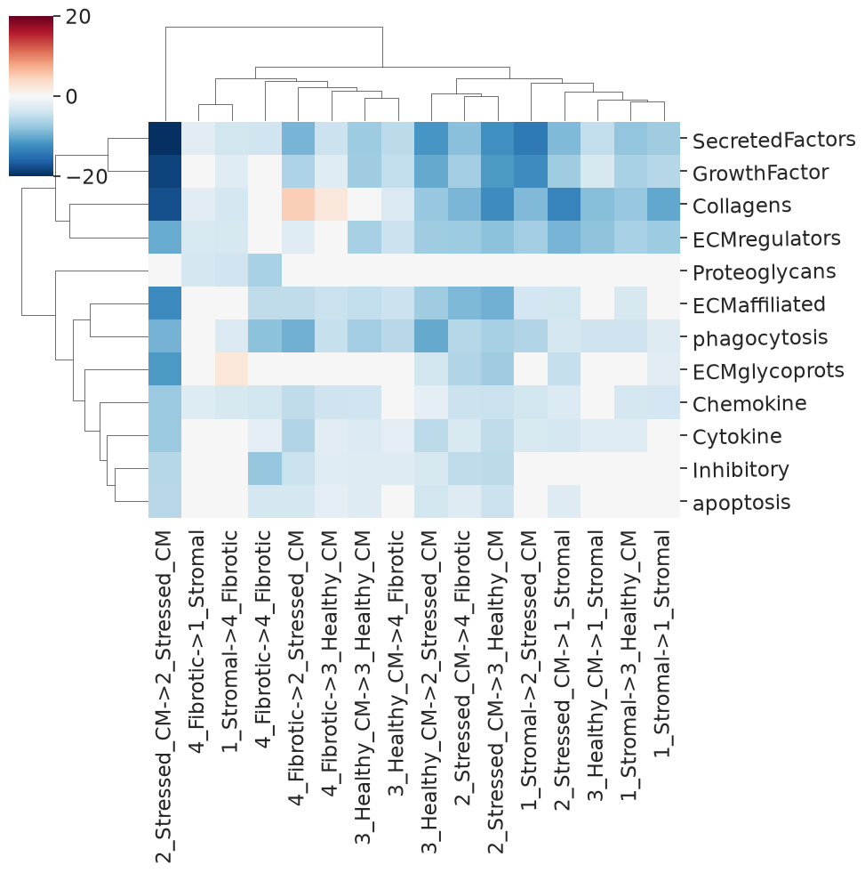
Differential communication per niche pair

diffCcommStats tests for differential communication per process using Wilcoxon rank-sum tests. Setting cellCatCol='niche_pairs' aggregates at the niche level for a high-level view:

diffComm_niches = nichesphere.comm.diffCcommStats(
    c1CTpairScores_byCat=iscCTpairScores,
    c2CTpairScores_byCat=myoCTpairScores,
    cellCatCol='niche_pairs'
)

hm_df, cm = nichesphere.comm.plotDiffCcommStatsHM(
    diffCommTable=diffComm_niches, min_pval=0.05, vmin=-20, vmax=20
)

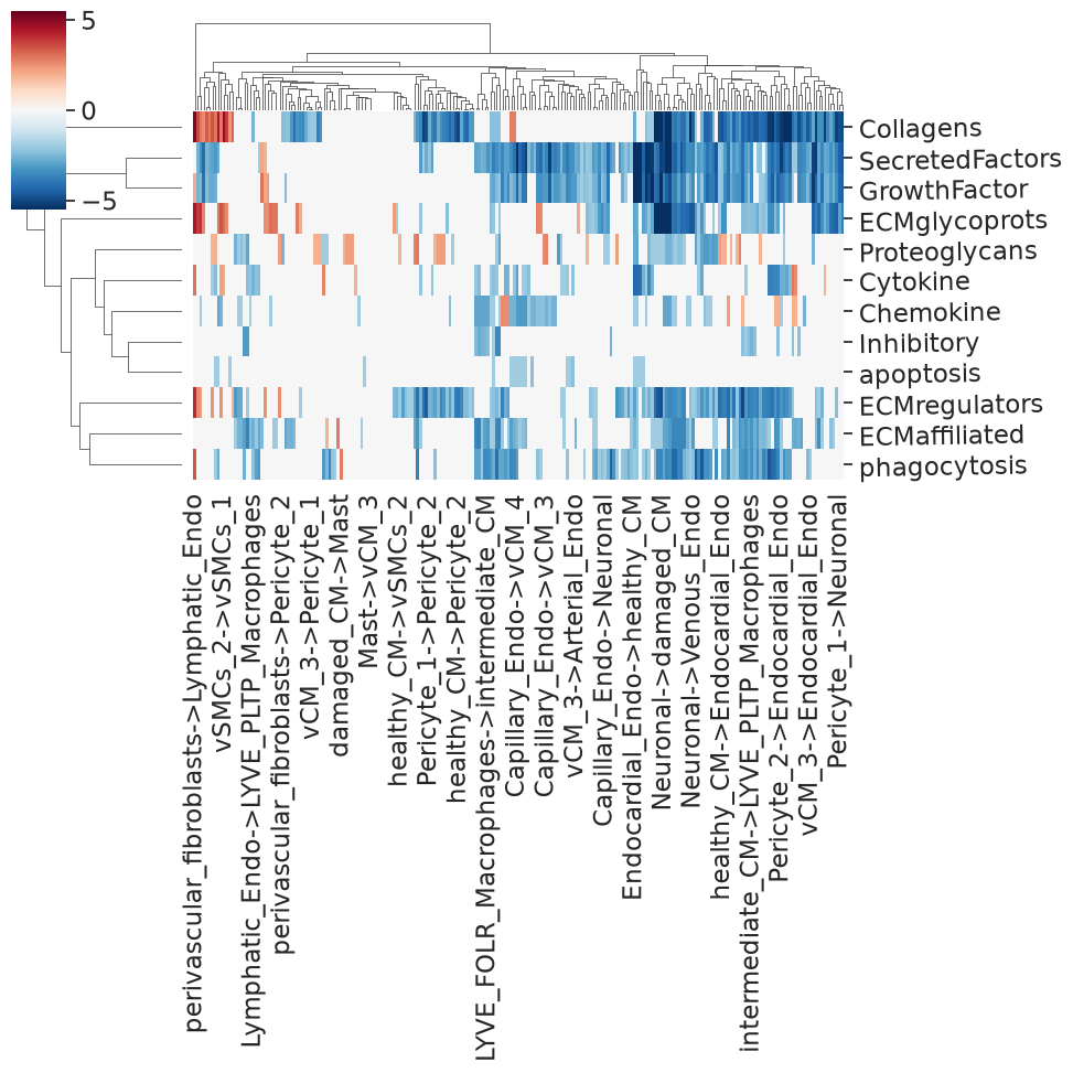
Differential communication per cell type pair

We repeat the test with cellCatCol='cell_pairs' to get cell-type-level resolution, needed to build process-specific communication networks:

diffComm_ctpairs = nichesphere.comm.diffCcommStats(
    c1CTpairScores_byCat=iscCTpairScores,
    c2CTpairScores_byCat=myoCTpairScores,
    cellCatCol='cell_pairs'
)

x_myoIsc_dir, _ = nichesphere.comm.plotDiffCcommStatsHM(
    diffCommTable=diffComm_ctpairs, min_pval=0.05, vmin=-5.5, vmax=5.5
)

11. Localized differential communication networks

getDiffComm extracts differential communication scores for a specific process, then catNW overlays these scores as edge weights on the co-localization network layout. We reload the saved network and node positions:

cat = 'ECMglycoprots'

x_chem = nichesphere.comm.getDiffComm(
    diffCommTbl=x_myoIsc_dir,
    pairCatDF=pairCatDFdir,
    ncells=33,
    cat=cat
)

plt.rcParams['axes.facecolor'] = 'None'
G = nichesphere.comm.catNW(
    x_chem=x_chem,
    colocNW=gCol,
    cell_group=niches_dict,
    plot_title=cat,
    clist=clist,
    nodeSize='betweeness',
    layout=None,
    #thr=5.5,
    fsize=(10, 10),
    #alpha=0.4,
    edge_scale=0.5,
    pos=pos,
    lab_spacing=0.05
)

legend_elements = [
    plt.Line2D([0], [0], marker='o', color='w', markerfacecolor=clist[i],
               lw=4, label=list(niches_dict.keys())[i], ms=10)
    for i in range(len(niches_dict))
]
plt.gca().add_artist(
    plt.legend(handles=legend_elements, loc='upper left', fontsize=13,
               title='Niches', alignment='left')
)
# plt.savefig(f'{cat}_diffCommNW.pdf')

<matplotlib.legend.Legend at 0x1553ffdaa2a0>

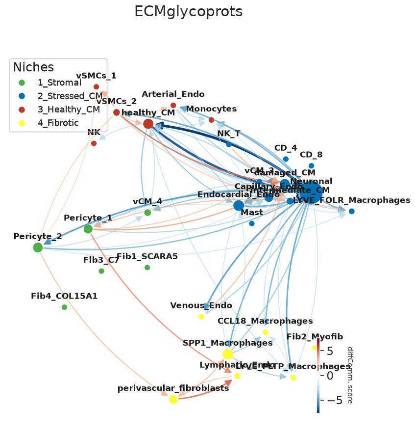
Network statistics for the communication network (note: G here is a directed graph, so we use in/out-degree):

comm_stats = nichesphere.tl.compute_network_stats(G)
comm_stats.head()

	betweenness	pagerank	degree_positive	degree_negative
Fib1_SCARA5	0.000000	1.244569	0.000000	0.000000
damaged_CM	-24.834053	2.135863	0.206897	0.103448
Capillary_Endo	-27.801873	-1.975055	0.000000	0.310345
LYVE_FOLR_Macrophages	0.000000	-0.594277	0.034483	0.172414
Fib3_C7	0.000000	1.244569	0.000000	0.000000

sns.set(font_scale=2)
plt.rcParams['axes.facecolor'] = 'None'
f=nichesphere.tl.plot_top_stats(comm_stats, top_n=5)

12. Sankey diagrams

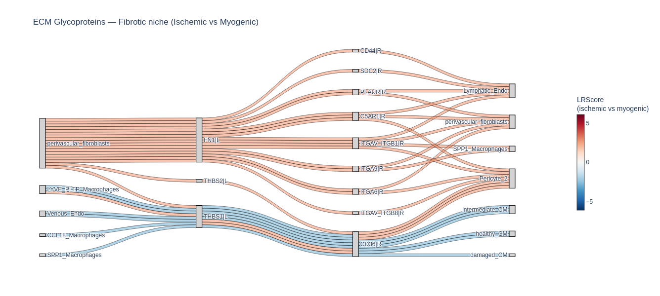
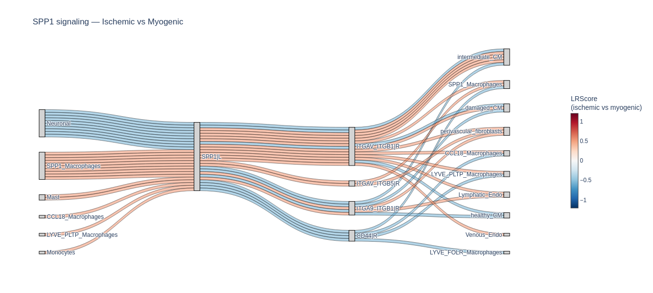
nichesphere.sankey_plot.plot_custom_sankey visualises differential LR communication as a four-layer Sankey diagram (source cell type → ligand → receptor → target cell type), built with Plotly. Links are colored by LR score (positive = red, negative = blue).

All filter arguments can be combined: only interactions satisfying all criteria are shown.

# All ECM glycoprotein interactions from fibrotic niche cell types
ECM_GPs = list(allDBs.Ligand[allDBs.category == 'ECMglycoprots'].str.lower())
fibrotic_cts = niches_dict['4_Fibrotic']

fig = nichesphere.sankey_plot.plot_custom_sankey(
    adata=adata_sc_raw,                   # pass None if using a pre-loaded table (see below)
    table_key='ischemic_x_myogenic',
    filter_df=colocFilt,
    source_cell=fibrotic_cts,
    ligand_list=ECM_GPs,
    threshold=25,
    title='ECM Glycoproteins — Fibrotic niche (Ischemic vs Myogenic)',
    # save_path='figures/fibrotic_ECMglycoprots_sankey.html'
)
fig.show()

Plotting 25 distinct fluid flow paths.

Filter to a specific ligand (e.g. SPP1) to trace all its interactions across conditions:

fig = nichesphere.sankey_plot.plot_custom_sankey(
    adata=adata_sc_raw,
    table_key='ischemic_x_myogenic',
    filter_df=colocFilt,
    ligand_gene='SPP1',
    threshold=25,
    title='SPP1 signaling — Ischemic vs Myogenic'
)
fig.show()

Plotting 25 distinct fluid flow paths.

---

This concludes the NicheSphere MI Visium tutorial. We have demonstrated:

• Computing cell type co-localization probabilities from Visium deconvolution data

• Testing differential co-localization across conditions and building a co-localization network

• Detecting niches with Louvain community detection and a community-aware layout

• Characterizing niche cohesion with nichesphere.niche_stats

• Computing process-based localized differential cell-cell communication from CrossTalkeR data

• Overlaying differential communication onto the co-localization network per process

• Visualizing specific LR interactions with interactive Sankey diagrams

For the PILOT trajectory inference integration, see the companion tutorial: Nichesphere_tutorial_MIvisium_PILOT.ipynb.

For further details on individual functions, see the NicheSphere documentation.