
NicheSphere tutorial (PIC-seq)#
NicheSphere is an sc-verse compatible Python library that identifies differentially co-localised cellular niches based on cell type pair co-localization probabilities across conditions. These probabilities are derived from deconvoluted spatial transcriptomics / PIC-seq data (i.e. the probability of finding each cell type in a given spot or multiplet), and are used to estimate the probability of finding each cell type pair together.
NicheSphere can also identify differentially communicating cellular niches based on Ligand-Receptor (LR) interaction data, such as the output of pyCrossTalkeR.
Finally, NicheSphere combines co-localization and communication networks into communication-weighted co-localization distances, enabling the identification of differentially interacting niches.
In this tutorial, we apply NicheSphere to this bone marrow fibrosis PIC-seq data to explore the bone marrow fibrosis-related cellular microenvironment. We will:
Load PIC-seq deconvolution results and the matching scRNA-seq data
Compute condition specific co-localization of cell type pairs
Build and explore a differential co-localization network, including niche detection
Compute process-based differential cell-cell communication (using CrossTalkeR output)
Combine co-localization and communication into localized differential communication networks
Visualize selected ligand-receptor relationships with Sankey diagrams
Please install the development version of NicheSphere directly from GitHub
```bash pip install git+https://github.com/CostaLab/NicheSphere@dev
1. Setup#
Import the libraries needed for this tutorial.
[1]:
import pandas as pd
import numpy as np
import scipy
import seaborn as sns
import matplotlib.pyplot as plt
import networkx as nx
import warnings
import scanpy as sc
import time
import nichesphere

warnings.filterwarnings("ignore")
NicheSphere also relies on two companion packages for parts of this tutorial:
pyCrossTalkeR to compute ligand-receptor communication scores per condition
community-layout to lay out community-detected networks
We import these where they are needed below.
2. Input data#
NicheSphere requires three inputs:
Cell type proportions per spot/multiplet, obtained by deconvoluting spatial transcriptomics or PIC-seq data with a method of choice (here we used BayesPrism, but any method returning a table of cell type proportions per spot/multiplet works).
scRNA-seq data (“singlets”) from the same biological system, used to build a background distribution for differential co-localization testing.
Spatial/multiplet (“doublet”) sequencing data, used to identify the conditions/samples present.
Cell type proportions in doublets/spots#
[2]:
CTprops = pd.read_csv('../../data/BM_PICseq/PICseq_doublets_CTprops.csv', index_col=0)
CTprops.head()
[2]:
| DC | InfiltMac | Fibro | MonoPro | Neut2 | Ly6ClowMac | Baso | TCells | Neut1 | MK | ResMac | OsteoCAR | EC | Ery | Spp1+Mac | BCells | |
|---|---|---|---|---|---|---|---|---|---|---|---|---|---|---|---|---|
| IS3_AAACCCAAGAGTCAGC-1 | 0.022321 | 0.009692 | 0.002134 | 0.019810 | 0.027176 | 0.005223 | 0.005350 | 0.006909 | 0.859264 | 0.013108 | 0.004198 | 0.002142 | 0.004581 | 0.008093 | 0.008558 | 0.001440 |
| IS3_AAACCCAAGGGCTGAT-1 | 0.009302 | 0.013937 | 0.003087 | 0.008581 | 0.013993 | 0.868811 | 0.012865 | 0.014621 | 0.009612 | 0.008361 | 0.005726 | 0.003589 | 0.009012 | 0.008289 | 0.008231 | 0.001982 |
| IS3_AAACCCACACGCCAGT-1 | 0.675809 | 0.260256 | 0.001310 | 0.006162 | 0.004601 | 0.005598 | 0.004135 | 0.005520 | 0.009202 | 0.010234 | 0.002177 | 0.001419 | 0.002356 | 0.006113 | 0.004108 | 0.001000 |
| IS3_AAACCCACACTACCGG-1 | 0.002942 | 0.003383 | 0.001131 | 0.850736 | 0.101740 | 0.002235 | 0.004787 | 0.002345 | 0.007967 | 0.005849 | 0.001834 | 0.001331 | 0.002962 | 0.003802 | 0.006055 | 0.000903 |
| IS3_AAACCCACAGATCCTA-1 | 0.030429 | 0.079342 | 0.005465 | 0.013012 | 0.047528 | 0.643361 | 0.025168 | 0.012989 | 0.035907 | 0.018483 | 0.043229 | 0.005768 | 0.010787 | 0.014002 | 0.010533 | 0.003997 |
The cell type probabilities should sum to 1 for each spot/multiplet:
[3]:
CTprops.sum(axis=1).head()
[3]:
IS3_AAACCCAAGAGTCAGC-1    1.0
IS3_AAACCCAAGGGCTGAT-1    1.0
IS3_AAACCCACACGCCAGT-1    1.0
IS3_AAACCCACACTACCGG-1    1.0
IS3_AAACCCACAGATCCTA-1    1.0
dtype: float64
scRNA-seq data (singlets)#
[4]:
adata_singlets = sc.read('../../data/BM_PICseq/PICseq_singlets.h5ad')
adata_singlets.obs.annotation = list(adata_singlets.obs.annotation)
Multiplet/spot sequencing data#
[5]:
adata_doublets = sc.read('../../data/BM_PICseq/PICseq_doublets.h5ad')
3. Differential co-localization analysis#
We first compute cell type pair co-localization probabilities from the deconvolution results using coloc.getColocProbs. This returns concatenated co-localization matrices (cell type x cell type) per sample, with the sample indicated in the last column.
[6]:
CTcolocalizationP = nichesphere.coloc.getColocProbs(CTprobs=CTprops, spotSamples=adata_doublets.obs.stage)
CTcolocalizationP.head()
[6]:
| DC | InfiltMac | Fibro | MonoPro | Neut2 | Ly6ClowMac | Baso | TCells | Neut1 | MK | ResMac | OsteoCAR | EC | Ery | Spp1+Mac | BCells | sample | |
|---|---|---|---|---|---|---|---|---|---|---|---|---|---|---|---|---|---|
| DC | 0.018899 | 0.003145 | 0.002420 | 0.009168 | 0.004171 | 0.001827 | 0.001256 | 0.003089 | 0.006253 | 0.005446 | 0.002721 | 0.001507 | 0.001714 | 0.006465 | 0.003841 | 0.000943 | EV |
| InfiltMac | 0.003145 | 0.007253 | 0.001322 | 0.003761 | 0.002179 | 0.001766 | 0.000631 | 0.001563 | 0.002736 | 0.001967 | 0.001844 | 0.000794 | 0.000946 | 0.002822 | 0.002009 | 0.000496 | EV |
| Fibro | 0.002420 | 0.001322 | 0.020764 | 0.005082 | 0.002962 | 0.001163 | 0.000904 | 0.001726 | 0.004088 | 0.002725 | 0.001727 | 0.002111 | 0.001767 | 0.004005 | 0.002702 | 0.000876 | EV |
| MonoPro | 0.009168 | 0.003761 | 0.005082 | 0.055366 | 0.011903 | 0.003358 | 0.002878 | 0.005730 | 0.016713 | 0.012703 | 0.004622 | 0.003131 | 0.003569 | 0.014315 | 0.007889 | 0.002072 | EV |
| Neut2 | 0.004171 | 0.002179 | 0.002962 | 0.011903 | 0.016147 | 0.002004 | 0.001496 | 0.003008 | 0.011881 | 0.004586 | 0.002610 | 0.001726 | 0.001901 | 0.007352 | 0.004330 | 0.001248 | EV |
We keep track of same-cell-type pairs (e.g. Fibro-Fibro), since these are typically excluded from downstream analyses:
[7]:
oneCTints = CTcolocalizationP.columns[:-1] + '-' + CTcolocalizationP.columns[:-1]
Next, we reshape the co-localization data into a matrix of cell type pairs x samples with coloc.reshapeColoc. Set complete=1 if your co-localization data contains both directions of a pair (ct1-ct2 and ct2-ct1); set complete=0 if it does not.
[8]:
colocPerSample = nichesphere.coloc.reshapeColoc(CTcoloc=CTcolocalizationP, complete=1)
colocPerSample
[8]:
| DC-DC | DC-InfiltMac | DC-Fibro | DC-MonoPro | DC-Neut2 | DC-Ly6ClowMac | DC-Baso | DC-TCells | DC-Neut1 | DC-MK | ... | BCells-Baso | BCells-TCells | BCells-Neut1 | BCells-MK | BCells-ResMac | BCells-OsteoCAR | BCells-EC | BCells-Ery | BCells-Spp1+Mac | BCells-BCells | |
|---|---|---|---|---|---|---|---|---|---|---|---|---|---|---|---|---|---|---|---|---|---|
| EV | 0.018899 | 0.003145 | 0.002420 | 0.009168 | 0.004171 | 0.001827 | 0.001256 | 0.003089 | 0.006253 | 0.005446 | ... | 0.000338 | 0.000741 | 0.001673 | 0.001140 | 0.000657 | 0.000472 | 0.000449 | 0.00168 | 0.001045 | 0.004976 |
| TPO | 0.043204 | 0.011930 | 0.000577 | 0.007006 | 0.002704 | 0.004632 | 0.001131 | 0.001506 | 0.005417 | 0.004213 | ... | 0.000112 | 0.000134 | 0.000347 | 0.000144 | 0.000150 | 0.000077 | 0.000050 | 0.00007 | 0.000078 | 0.000504 |
2 rows × 256 columns
Co-localization probabilities of all cell type pairs should sum to 1 per sample:
[9]:
colocPerSample.sum(axis=1)
[9]:
EV     1.0
TPO    1.0
dtype: float64
Background distribution and observed vs. expected ratios#
In this dataset we do not have replicate samples per condition, so we test differential co-localization by comparing observed co-localization probabilities to a background distribution. The background is generated by randomly pairing cells from the scRNA-seq (singlets) data of the same condition to form synthetic “doublets”, and computing the resulting observed/expected (O/E) co-localization ratios. By default we generate 1000 random background doublet sets per cell type pair.
Building the background distribution#
We compute the background distribution from the singlets data of the TPO condition. Here, the cell type proportions in the gated singlets data were biased (Fibroblast and OsteoCAR cells were over-represented), so we downsample these two cell types by a factor of 6 to better reflect their true in-tissue proportions before sampling random doublets.
[10]:
t = time.time()
res = nichesphere.tl.get_PIC_BG_OEratios_DF(
    adata=adata_singlets[adata_singlets.obs.stage == 'TPO'],
    annot_col='annotation',
    target_pairs=colocPerSample.columns,
    nreps=1000,
    njobs=10,
    downsample_cells=True,
    cell_list_downsample=['Fibro', 'OsteoCAR'],
    downsampling_factor=6,
)
bg_df = res  # get_PIC_BG_OEratios_DF already returns the concatenated DataFrame
print(time.time() - t)
45.86140990257263
45.8991425037384
[11]:
bg_df.head()
[11]:
| DC-DC | DC-InfiltMac | DC-Fibro | DC-MonoPro | DC-Neut2 | DC-Ly6ClowMac | DC-Baso | DC-TCells | DC-Neut1 | DC-MK | ... | BCells-Baso | BCells-TCells | BCells-Neut1 | BCells-MK | BCells-ResMac | BCells-OsteoCAR | BCells-EC | BCells-Ery | BCells-Spp1+Mac | BCells-BCells | |
|---|---|---|---|---|---|---|---|---|---|---|---|---|---|---|---|---|---|---|---|---|---|
| OE_Ratio | 0.947224 | 1.060056 | 5.559794e-11 | 1.236195 | 0.929457 | 0.890595 | 1.103392 | 1.350236 | 0.860871 | 1.133869 | ... | 1.863945e-10 | 3.756832e-10 | 1.696634e-10 | 5.959113e-10 | 1.362275e+00 | 1.344111e-08 | 6.235567e-10 | 2.240185e-09 | 8.064667e-09 | 6.366842e-09 |
| OE_Ratio | 1.380241 | 0.983656 | 5.947687e-11 | 1.094337 | 0.899474 | 1.079748 | 0.906358 | 1.191384 | 1.004350 | 0.503942 | ... | 1.863945e-10 | 3.756832e+00 | 1.696634e-10 | 5.959113e-10 | 1.362275e-10 | 1.008083e-08 | 6.235567e-10 | 2.240185e-09 | 8.064667e-09 | 6.366842e-09 |
| OE_Ratio | 0.920161 | 1.021856 | 5.947687e-11 | 0.770089 | 0.989422 | 0.969409 | 1.024578 | 0.397128 | 0.609784 | 1.511826 | ... | 1.863945e+00 | 3.756832e-10 | 1.696634e+00 | 5.959113e+00 | 1.362275e+00 | 1.008083e-08 | 6.235567e-10 | 2.240185e-09 | 8.064667e+01 | 6.366842e-09 |
| OE_Ratio | 0.974288 | 1.193757 | 6.089298e-11 | 1.155133 | 1.169317 | 1.087629 | 0.709323 | 0.953108 | 1.076089 | 1.511826 | ... | 3.727889e+00 | 3.756832e-10 | 1.696634e-10 | 5.959113e+00 | 1.362275e-10 | 9.305385e-09 | 6.235567e+00 | 2.240185e-09 | 8.064667e-09 | 6.366842e+01 |
| OE_Ratio | 1.244923 | 1.069606 | 5.441501e-11 | 0.871416 | 1.079369 | 0.969409 | 1.497461 | 0.555979 | 0.896741 | 0.881898 | ... | 1.863945e+00 | 3.756832e-10 | 1.696634e+00 | 5.959113e-10 | 1.362275e-10 | 1.512125e-08 | 6.235567e+00 | 2.240185e-09 | 8.064667e-09 | 6.366842e-09 |
5 rows × 256 columns
We apply the same downsampling to the singlets cell type list before computing expected co-localization probabilities, so that observed and expected probabilities are on the same scale:
[12]:
TPO_cell_list = list(adata_singlets[adata_singlets.obs.stage == 'TPO'].obs['annotation'])
TPO_cell_list = nichesphere.tl.downsample_class(TPO_cell_list, target_class=['Fibro', 'OsteoCAR'], factor=6)
TPO_cell_series = pd.Series(TPO_cell_list)
Expected co-localization probabilities#
We compute the expected probability of each cell type pair occurring in this condition, based on cell type proportions in the (downsampled) singlets data:
[13]:
scCTpairsProbs_TPO = nichesphere.tl.getExpectedColocProbsFromSCs(annot_series=TPO_cell_series, cell_types=CTprops.columns)
scCTpairsProbs_TPO.head()
[13]:
| count | |
|---|---|
| DC-DC | 0.006115 |
| DC-InfiltMac | 0.017312 |
| DC-Fibro | 0.000272 |
| DC-MonoPro | 0.008158 |
| DC-Neut2 | 0.005514 |
Differential co-localization scores#
We now compute log2(observed/expected) ratios, filtering out non-significant values (here p=0.1) and same-cell-type interactions, using OvsE_coloc_test. We can visualize the resulting scores in a heatmap, clustering cell types by their differential co-localization profiles.
[14]:
OvsE_TPO_HMdf, stats = nichesphere.coloc.OvsE_coloc_test_adjPval(
    observedColocProbs=colocPerSample.loc['TPO'],
    expectedColocProbs=scCTpairsProbs_TPO['count'],
    cell_types=CTprops.columns,
    testDistribution_df=bg_df,
    oneCTinteractions=oneCTints,
    p=0.1
)

sns.set(font_scale=1)
sns.clustermap(OvsE_TPO_HMdf, cmap='RdBu_r', center=0, method='ward', cbar_kws={'label': 'diffColoc. Score'})
[14]:
<seaborn.matrix.ClusterGrid at 0x1554eb73c290>

OvsE_coloc_test also returns the underlying statistics:
[15]:
stats.head()
[15]:
| statistic | pvalue | adjusted_pvalue | |
|---|---|---|---|
| DC-DC | 0.000000 | 0.000 | 0.000000 |
| DC-InfiltMac | -0.537164 | 0.000 | 0.000000 |
| DC-Fibro | 1.088154 | 0.000 | 0.000000 |
| DC-MonoPro | 0.000000 | 0.258 | 0.313024 |
| DC-Neut2 | -1.028178 | 0.002 | 0.003200 |
[16]:
#stats.to_csv('../tutorial_results/diffcoloc_stats.csv')
4. Differential co-localization network#
To build the differential co-localization network, we compute an adjacency matrix based on the Euclidean distances between the differential co-localization profiles of each cell type.
[17]:
HMdist = pd.DataFrame(
    scipy.spatial.distance.squareform(scipy.spatial.distance.pdist(OvsE_TPO_HMdf)),
    columns=OvsE_TPO_HMdf.columns, index=OvsE_TPO_HMdf.index
)

HMsimm = 1 - HMdist / HMdist.max().max()
# Cell pairs with no significant differential co-localization get 0
HMsimm[OvsE_TPO_HMdf == 0] = 0
[18]:
sns.set(font_scale=1)
sns.clustermap(HMsimm, cmap='Blues', method='ward', cbar_kws={'label': 'adjacency'})
[18]:
<seaborn.matrix.ClusterGrid at 0x1554eb39d910>

Niche detection#
Before clustering the network into niches, we use a single placeholder group/color so that the initial network can be plotted with coloc.colocNW. The network is built from the differentially co-localized cell type pairs only.
[19]:
plt.rcParams['axes.facecolor'] = "None"

niches_dict = {'1_': list(OvsE_TPO_HMdf.index)}
clist = ['#4daf4a']

gCol = nichesphere.coloc.colocNW(x_diff=OvsE_TPO_HMdf, adj=HMsimm, cell_group=niches_dict,
                                  clist=clist, nodeSize='betweeness', layout='neato', thr=0)

We then detect communities (niches) in the unsigned network using Louvain clustering:
[20]:
gCol2 = nx.from_pandas_adjacency(HMsimm, create_using=nx.Graph)

niches_raw = nx.algorithms.community.louvain_communities(gCol2, resolution=1.2, seed=1, weight='weight')
niches_dict = dict(enumerate([list(x) for x in niches_raw]))
niches_dict
[20]:
{0: ['ResMac', 'DC', 'Neut2', 'Baso'],
 1: ['MK', 'TCells', 'Ery', 'Spp1+Mac', 'OsteoCAR'],
 2: ['Ly6ClowMac', 'EC', 'InfiltMac'],
 3: ['Fibro', 'Neut1', 'BCells', 'MonoPro']}
We can give the detected niches descriptive names and assign each a color for visualization:
[21]:
#niche_names = ['1_Neut_ResMac_Baso_DC', '2_FibCore', '3_Macs_EC', '4_BCells_Fibro']
niche_names=['1_Resident_myeloid_niche', '2_FibCore', '3_Macrophage_vascular_niche', '4_Fibro_myeloid_niche']
niches_dict = dict(zip(niche_names, list(niches_dict.values())))

clist = ['#FF8C00', '#32CD32', '#E64B35', '#FFD700']
niche_cols = pd.Series(clist, index=list(niches_dict.keys()))
niches_df = nichesphere.tl.cells_niche_colors(CTs=CTprops.columns, niche_colors=niche_cols, niche_dict=niches_dict)
Network layout#
We use the community-layout package’s CommunityLayout to lay out the network so that niches (communities) are visually grouped together. CommunityLayout is compatible with NetworkX (Hagberg et al., 2008) community detection functions, used internally via the community_algorithm and community_kwargs parameters.
[22]:
from community_layout.layout_class import CommunityLayout

cl = CommunityLayout(
    gCol2,
    community_compression=0.4,
    layout_algorithm=nx.spring_layout,
    layout_kwargs={"k": 75, "iterations": 1000},
    community_algorithm=nx.algorithms.community.louvain_communities,
    community_kwargs={"resolution": 1.2, 'seed': 1, 'weight': 'weight'}
)

pos = cl.full_positions
COMMUNITY LAYOUT: Datashader not found, edge bundling not available
Building meta-graph
Metagraph is a Graph with 4 nodes and 6 edges
100%|██████████| 4/4 [00:00<00:00, 470.78it/s]
We can now plot the differential co-localization network with niches highlighted by color, using the community-aware layout:
[23]:
# Load node positions
pos = np.load('../../data/BM_PICseq/diffColocNW_node_pos.npy',allow_pickle='TRUE').item()
[24]:
gCol = nichesphere.coloc.colocNW(
    x_diff=OvsE_TPO_HMdf,
    adj=HMsimm,
    cell_group=niches_dict,
    clist=clist,
    nodeSize='betweeness',
    layout=None,  # set to None when providing node positions
    lab_spacing=0.05,
    thr=0,
    pos=pos,
    edge_scale=0.7,
    legend_ax=[0.05, 0.75, 0.15, 0.2]
)

legend_elements = [
    plt.Line2D([0], [0], marker="o", color='w', markerfacecolor=clist[i], lw=4,
               label=list(niches_dict.keys())[i], ms=10)
    for i in range(len(niches_dict))
]
plt.gca().add_artist(plt.legend(handles=legend_elements, loc='lower right', fontsize=13,
                                 title='Niches', alignment='left'))

#plt.savefig('../figures/diffColocNW.pdf')
[24]:
<matplotlib.legend.Legend at 0x1553aaed3d40>

[25]:
## Save node positions
#np.save('../tutorial_data/diffColocNW_node_positions.npy', pos)
Finally, we assign niche/community information and node positions to the network object, so they can be reused for subsequent network visualizations:
[26]:
nichesphere.tl.assign_properties(
    gCol,
    communities=cl.communities(),
    colors=clist,
    pos=pos,
    simmilarity_weights=True,
    node_coord_sf=100,
    g_unsigned=gCol2
)
Interactive network#
The gravis library enables an interactive D3-based network visualization where node sizes, edge widths, and label sizes can be adjusted in the browser. One can also move the nodes around to avoid overlaps.
Note: gravis may require downgrading setuptools:
pip install --force-reinstall -U "setuptools<82.0.0"
[27]:
import gravis as gv
gv.d3(gCol, edge_size_data_source='weight_abs', zoom_factor=0.35, layout_algorithm_active=False)
[27]:
Network statistics#
We can compute and visualize standard network statistics (betweenness centrality, PageRank, and degree centrality split by positive/negative edges). These are based on the implementations from NetworkX:
[28]:
nw_stats = nichesphere.tl.compute_network_stats(gCol)
nw_stats.head()
[28]:
| betweenness | pagerank | degree_positive | degree_negative | |
|---|---|---|---|---|
| DC | 22.697681 | -1.020317 | 0.333333 | 0.333333 |
| InfiltMac | -6.489179 | -2.196781 | 0.266667 | 0.600000 |
| Fibro | 30.776810 | 2.731931 | 0.933333 | 0.000000 |
| MonoPro | 22.697681 | -1.134020 | 0.400000 | 0.266667 |
| Neut2 | 22.697681 | -1.056960 | 0.333333 | 0.333333 |
[29]:
#nw_stats.to_csv('../tutorial_results/diffColocNW_stats.csv')
[30]:
sns.set(font_scale=2)
plt.rcParams['axes.facecolor'] = "None"
fig = nichesphere.tl.plot_top_stats(nw_stats, top_n=5)
#plt.savefig('../figures/diffColocNW_stats_top5.pdf')

Niche cohesion: internal vs external edge weights#
To assess how cohesive each detected niche is, we compare the distribution of co-localization scores for edges connecting cell types within the same niche (internal) against edges connecting cell types across niches (external). A niche with predominantly positive internal edges and weaker or negative external edges is more tightly co-localized internally than expected by chance.
We first build a partition map from the Louvain community detection result, then use nichesphere.niche to visualise and test the distributions.
[31]:
# Map each cell type node to its named niche
d = nx.algorithms.community.louvain_communities(gCol2, resolution=1.2, seed=1, weight='weight')
vc_map = {node: i for i, members in enumerate(d) for node in members}

community_names = dict(enumerate(niche_names))  # reuse the niche_names list defined above
vc_map_named = {node: community_names[comm_id] for node, comm_id in vc_map.items()}
[32]:
sns.set(font_scale=1)
plt.rcParams['axes.facecolor'] = "None"
nichesphere.niche_stats.plot_internal_external_boxplots(gCol, vc_map_named)
#plt.savefig('../figures/diffColocNW_int_ext_boxplots.pdf', bbox_inches='tight')
[32]:
<Axes: title={'center': 'Internal vs external edge weight distributions by niche'}, xlabel='niche', ylabel='edge weight'>

We can also obtain a flat summary table of edge counts and total weights per niche:
[33]:
nichesphere.niche_stats.community_edge_stats_df(gCol, vc_map_named)
[33]:
| internal_pos_count | internal_pos_weight | internal_neg_count | internal_neg_weight | external_pos_count | external_pos_weight | external_neg_count | external_neg_weight | |
|---|---|---|---|---|---|---|---|---|
| community | ||||||||
| 1_Resident_myeloid_niche | 0 | 0.000000 | 6 | 10.646399 | 17 | 38.125336 | 13 | 21.593805 |
| 2_FibCore | 10 | 47.617059 | 0 | 0.000000 | 33 | 100.060348 | 3 | 3.114141 |
| 3_Macrophage_vascular_niche | 0 | 0.000000 | 3 | 3.609690 | 10 | 23.011103 | 14 | 23.687616 |
| 4_Fibro_myeloid_niche | 5 | 9.061479 | 0 | 0.000000 | 22 | 60.038467 | 8 | 13.486342 |
Finally, we test whether the internal and external edge weight distributions differ significantly for each niche using a Wilcoxon rank-sum test with FDR correction:
[34]:
signed        = nichesphere.niche_stats.community_signed_weight_distributions(gCol, vc_map_named)
communities   = sorted(signed.keys())
internal_data = [signed[c]['internal'] for c in communities]
external_data = [signed[c]['external'] for c in communities]

nichesphere.niche_stats.pairwise_ranksums_int_ext(
    internal_data, external_data, communities, MTcorrection='fdr_bh'
)
[34]:
| niche | statistic | p_value | p_value_corrected | |
|---|---|---|---|---|
| 0 | 1_Resident_myeloid_niche | -2.334620 | 0.019563 | 0.039127 |
| 1 | 2_FibCore | 2.743012 | 0.006088 | 0.024351 |
| 2 | 3_Macrophage_vascular_niche | -0.308607 | 0.757621 | 0.850436 |
| 3 | 4_Fibro_myeloid_niche | 0.188562 | 0.850436 | 0.850436 |
5. Process-based localized differential communication#
One of Nichesphere’s key features is process-based localized differential communication testing: looking at how ligand-receptor (LR) interactions belonging to specific biological processes change between niches across conditions.
To do this, we first need per-condition LR communication scores. We compute these by running LIANA and pyCrossTalkeR on the raw singlets data.
Preparing raw singlets data#
The deconvolution/annotation steps above used processed data. For LR analysis we use the corresponding raw count matrix and store it in a new anndata object with the metadata to avoid changes in the already processed data:
[35]:
import anndata as ad

adata_singlets_raw = ad.AnnData(
    X=adata_singlets.layers['counts'],
    obs=adata_singlets.obs,
    var=adata_singlets.var
)
adata_singlets_raw.raw = adata_singlets_raw
Running LIANA and pyCrossTalkeR#
For each condition, we compute LR interaction scores with LIANA’s CellPhoneDB method, then convert the results into pyCrossTalkeR format and run the differential analysis between conditions:
[36]:
import os
from pycrosstalker import tools as cttl
import liana as li

#adata_singlets_raw.raw = adata_singlets_raw

adata_singlets_raw.uns['liana'] = {}
for stage in set(adata_singlets_raw.obs['stage']):
    lr = li.method.cellphonedb(
        adata_singlets_raw[adata_singlets_raw.obs['stage'] == stage],
        groupby='annotation',
        expr_prop=0.1,
        verbose=True,
        resource_name='mouseconsensus',
        inplace=False
    )
    adata_singlets_raw.uns['liana'][stage] = lr

adata_singlets_raw = cttl.utils.from_liana(adata_singlets_raw)
adata_singlets_raw.uns['pycrosstalker']['details'] = {'filename': 'PICseq'}

output = './results/output_ctkr/PICseq/'
os.makedirs(output, exist_ok=True)
adata_singlets_raw = cttl.analise_LR(adata_singlets_raw, out_path=output, comparison=[('TPO', 'EV')])
Using resource `mouseconsensus`.
Using `.raw`!
Converting to sparse csr matrix!
1129 features of mat are empty, they will be removed.
Converting `annotation` to categorical!
0.30 of entities in the resource are missing from the data.
Generating ligand-receptor stats for 12373 samples and 1070 features
100%|██████████| 1000/1000 [00:47<00:00, 20.85it/s]
Using resource `mouseconsensus`.
Using `.raw`!
Converting to sparse csr matrix!
1104 features of mat are empty, they will be removed.
Converting `annotation` to categorical!
0.28 of entities in the resource are missing from the data.
Generating ligand-receptor stats for 14673 samples and 1084 features
100%|██████████| 1000/1000 [00:44<00:00, 22.42it/s]
Create a Differential Table
Calculating CCI Ranking
Calculating GCI Ranking
... storing 'annotation' as categorical
Network Analysis Done
Generating h5ad file with Analysed Results
Mapping cell type pairs to niche pairs#
Next we assign each cell type pair to its corresponding niche pair, so that communication scores can later be aggregated and compared at the niche level:
[37]:
oneCTints = pd.Series(oneCTints)
pairCatDFdir = nichesphere.tl.get_pairCatDFdir(niches_df)
pairCatDFdir.head()
[37]:
| cell_pairs | niche_pairs | |
|---|---|---|
| 0 | DC->DC | 1_Resident_myeloid_niche->1_Resident_myeloid_n... |
| 1 | DC->InfiltMac | 1_Resident_myeloid_niche->3_Macrophage_vascula... |
| 2 | DC->Fibro | 1_Resident_myeloid_niche->4_Fibro_myeloid_niche |
| 3 | DC->MonoPro | 1_Resident_myeloid_niche->4_Fibro_myeloid_niche |
| 4 | DC->Neut2 | 1_Resident_myeloid_niche->1_Resident_myeloid_n... |
Filtering by co-localization#
We restrict communication testing to cell type pairs with significant differential co-localization scores. Pairs with filter==1 will be tested downstream:
[38]:
colocFilt = nichesphere.tl.getColocFilter(pairCatDF=pairCatDFdir, adj=HMsimm,
                                           oneCTints=oneCTints.str.replace('-', '->'))
#colocFilt.to_csv('../tutorial_results/colocFilt.csv')
colocFilt.head()
[38]:
| filter | |
|---|---|
| cell_pairs | |
| DC->DC | 1.0 |
| DC->InfiltMac | 1.0 |
| DC->Fibro | 1.0 |
| DC->MonoPro | 0.0 |
| DC->Neut2 | 1.0 |
CrossTalkeR communication tables#
We retrieve the per-condition LR communication tables produced by pyCrossTalkeR. These contain a cellpair column (cell types involved, separated by @), an allpair column (cell types, ligand, and receptor), and columns for the ligand (gene_A), receptor (gene_B), and communication score (MeanLR). Column names can be customized in NicheSphere functions if your data differs.
CrossTalkeR tables also annotate genes as ligand (|L), receptor (|R), or transcription factor (|TF); we remove these suffixes as they can conflict with downstream code.
[39]:
crossTalker_ctrlComm = adata_singlets_raw.uns['pycrosstalker']['path']['EV']
crossTalker_tpoComm = adata_singlets_raw.uns['pycrosstalker']['path']['TPO']

crossTalker_ctrlComm = nichesphere.tl.processCTKRoutput(crossTalker_ctrlComm)
crossTalker_tpoComm = nichesphere.tl.processCTKRoutput(crossTalker_tpoComm)
Ligand-process database#
To test differential communication per biological process, we load a database linking ligands to the processes they are involved in (compiled from several published ligand-receptor databases):
[40]:
import nichesphere.database as db
[41]:
# Load database
allDBs = db.load_DB()
[42]:
allDBs['Ligand'] = allDBs['Ligand'].str.lower()
allDBs.head()
[42]:
| Ligand | category | db | PMID | |
|---|---|---|---|---|
| 2 | col1a1 | Collagens | matrisome | 36399478 |
| 3 | col1a2 | Collagens | matrisome | 36399478 |
| 4 | col1a1 | Collagens | matrisome | 36399478 |
| 5 | col6a3 | Collagens | matrisome | 36399478 |
| 6 | col1a2 | Collagens | matrisome | 36399478 |
[43]:
allDBs_sub = allDBs[~allDBs.category.isin(['apoptosis', 'phagocytosis'])]
allDBs_sub = allDBs_sub.drop_duplicates()
[44]:
sns.set_context(rc={'patch.linewidth': 0.0})
sns.barplot(x=allDBs_sub.category.value_counts(), y=allDBs_sub.category.value_counts().index,
            data=pd.DataFrame(allDBs_sub.category.value_counts()), color='black')
sns.despine()

6. Differential communication testing#
We now split communication scores by process, to determine which cell type pairs (and niche pairs) are communicating through which processes, in each condition. Interactions present in only one condition are assigned a score of 0 in the other, so conditions can be compared directly.
[45]:
EV_scores = nichesphere.comm.lr_ctPairScores_perCat_dir(
    ccommTable=crossTalker_ctrlComm, db=allDBs_sub, dbCatCol='category', dbMatchCol='Ligand',
    ccommMatchCol='gene_A', ccommLRscoresCol='MeanLR',
    oneCTinteractions=oneCTints.str.replace('-', '@'), condition='EV', pairCatDF=pairCatDFdir
)

TPO_scores = nichesphere.comm.lr_ctPairScores_perCat_dir(
    ccommTable=crossTalker_tpoComm, db=allDBs_sub, dbCatCol='category', dbMatchCol='Ligand',
    ccommMatchCol='gene_A', ccommLRscoresCol='MeanLR',
    oneCTinteractions=oneCTints.str.replace('-', '@'), condition='TPO', pairCatDF=pairCatDFdir
)

EV_scores, TPO_scores = nichesphere.comm.equalizeScoresTables(
    ctrlTbl=EV_scores, expTbl=TPO_scores, ctrlCondition='EV', expCondition='TPO'
)
We then keep only the cell type pairs that passed the co-localization filter computed earlier:
[46]:
sig_pairs = colocFilt.index[colocFilt['filter'] == 1]
EV_scores = EV_scores[[i in sig_pairs for i in EV_scores.cell_pairs]]
TPO_scores = TPO_scores[[i in sig_pairs for i in TPO_scores.cell_pairs]]

TPO_scores.LRcat.value_counts()
[46]:
LRcat
SecretedFactors    1999
ECMregulators      1453
ECMglycoprots      1366
GrowthFactor       1190
Cytokine            918
Collagens           679
ECMaffiliated       620
Proteoglycans       275
Chemokine           265
Inhibitory          151
Name: count, dtype: int64
Differential communication per niche pair#
comm.diffCcommStats tests for differential communication between groups of interactions across processes. Setting cellCatCol='niche_pairs' aggregates results at the niche-pair level:
[47]:
diffComm_niches = nichesphere.comm.diffCcommStats(
    c1CTpairScores_byCat=TPO_scores, c2CTpairScores_byCat=EV_scores, cellCatCol='niche_pairs'
)
[48]:
hm_df, _ = nichesphere.comm.plotDiffCcommStatsHM(diffCommTable=diffComm_niches, min_pval=0.05)
hm_df = hm_df.T[hm_df.sum() != 0].T

cm = sns.clustermap(hm_df.T.sort_index(), cmap='RdBu_r', center=0, method='complete',
                     row_cluster=False, vmin=-5, vmax=5)
plt.setp(cm.ax_heatmap.yaxis.get_majorticklabels(), rotation=1, fontsize=8)
plt.setp(cm.ax_heatmap.xaxis.get_majorticklabels(), fontsize=8)

# Tidy up the figure layout
hm = cm.ax_heatmap.get_position()
cm.ax_heatmap.set_position([hm.x0, hm.y0, hm.width * 0.5, hm.height * 0.45])
col = cm.ax_col_dendrogram.get_position()
cm.ax_col_dendrogram.set_position([col.x0, col.y0 * 0.6, col.width * 0.5, col.height * 0.25])
row = cm.ax_row_dendrogram.get_position()
cm.ax_row_dendrogram.set_position([row.x0 * 3.5, row.y0, row.width * 0.2, row.height * 0.45])
x0, y0, w, h = cm.cbar_pos
cm.ax_cbar.set_position([x0 * 2.5, y0 * 0.63, w * 0.25, h * 0.3])
cm.tick_params(labelsize=8)

#plt.savefig('../figures/diffComm_byNichePair_byProcess.pdf')
plt.show()


Differential communication per cell type pair#
To build process-specific differential communication networks, we repeat the test with cellCatCol='cell_pairs', giving differential communication scores per cell type pair (rather than per niche pair):
[49]:
diffComm_ctpairs = nichesphere.comm.diffCcommStats(
    c1CTpairScores_byCat=TPO_scores, c2CTpairScores_byCat=EV_scores, cellCatCol='cell_pairs'
)

x_EVtpo_dir, _ = nichesphere.comm.plotDiffCcommStatsHM(diffCommTable=diffComm_ctpairs, min_pval=0.1)

7. Localized differential communication networks#
We can now overlay process-specific differential communication scores onto the co-localization network: for each process category, edges represent differential communication between niches/cell types, computed with comm.getDiffComm and visualized with comm.catNW.
Single-process network: example#
To produce a polished figure for a single process (e.g. ECMglycoprots), we plot the network using the saved community-aware layout (pos):
[50]:
plt.rcParams['axes.facecolor'] = "None"
[51]:
cat = 'ECMglycoprots'
x_chem = nichesphere.comm.getDiffComm(diffCommTbl=x_EVtpo_dir, pairCatDF=pairCatDFdir, ncells=16, cat=cat)

G = nichesphere.comm.catNW(x_chem=x_chem, colocNW=gCol, cell_group=niches_dict, group_cmap='tab20',
                            ncols=20, plot_title=cat, clist=clist, nodeSize='betweeness',
                            legend_ax=[0.0, 0.87, 0.15, 0.2], pos=pos, thr=0, layout=None, lab_spacing=0.05)

legend_elements = [
    plt.Line2D([0], [0], marker="o", color='w', markerfacecolor=clist[i], lw=4,
               label=list(niches_dict.keys())[i], ms=10)
    for i in range(len(niches_dict))
]
plt.gca().add_artist(plt.legend(handles=legend_elements, loc='lower right', fontsize=13,
                                 title='Niches', alignment='left'))
#plt.savefig(f'../figures/commNW_{cat}.pdf')
[51]:
<matplotlib.legend.Legend at 0x15539b33abd0>

[52]:
nw_stats_cat = nichesphere.tl.compute_network_stats(G)

sns.set(font_scale=2)
plt.rcParams['axes.facecolor'] = "None"
fig = nichesphere.tl.plot_top_stats(nw_stats_cat, top_n=5)
#plt.savefig(f'../figures/commNW_{cat}_stats_top5.pdf', bbox_inches='tight')

8. Visualizing ligand-receptor interactions with Sankey diagrams#
Finally, we can visualize selected ligand-receptor relationships as Sankey diagrams using pyCrossTalkeR’s results and NicheSphere’s sankey_plot module, for cell type pairs/processes of interest.
We start from the differential communication table (TPO_x_EV), restricted to the co-localization-filtered cell type pairs:
Example 1: Spp1 signaling from Spp1+ macrophages:
[53]:
fig2=nichesphere.sankey_plot.plot_custom_sankey(
    adata=adata_singlets_raw,
    table_key='TPO_x_EV',
    filter_df=colocFilt,
    source_cell='Spp1+Mac',
    ligand_gene='Spp1',
    threshold=25,
    title="Flat 2D Parallel Flow Map (Spp1 Paths)",
    #save_path="spp1Macs_spp1_sankey.pdf"
)
fig2.show()
Plotting 25 distinct fluid flow paths.

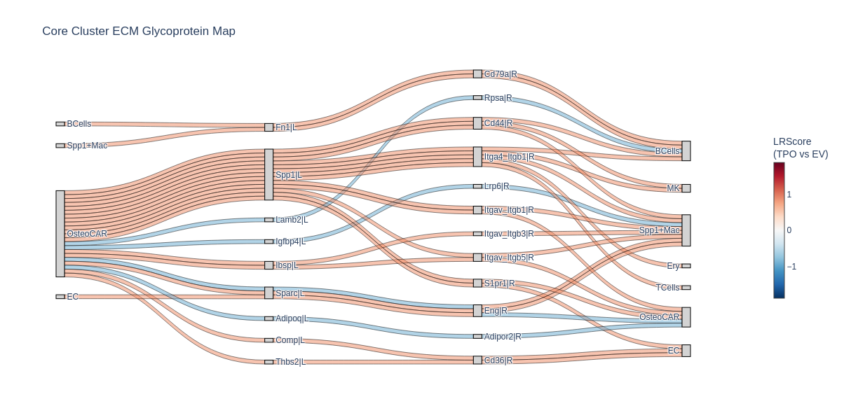
Example 2: ECM glycoprotein signaling within the fibrotic core niche:
[54]:
# Setup variables
ECM_GPs = list(allDBs_sub.Ligand[allDBs_sub.category == 'ECMglycoprots'])
fibCore = ['Spp1+Mac', 'BCells', 'MK', 'TCells', 'EC', 'OsteoCAR', 'Ery']

# Generate chart inline and save vector out
fig = nichesphere.sankey_plot.plot_custom_sankey(
    adata=adata_singlets_raw,
    table_key='TPO_x_EV',
    filter_df=colocFilt,
    source_cell=fibCore,
    target_cell=fibCore,
    ligand_list=ECM_GPs,
    threshold=25,
    title="Core Cluster ECM Glycoprotein Map",
    #save_path="fibCore_ECMglycoprots_sankey.pdf" # <-- Bypasses Python bugs and downloads vector directly via browser!
)
fig.show()
Plotting 25 distinct fluid flow paths.
This concludes the tutorial. We have shown how to:
Compute cell type pair co-localization probabilities from spatial/PIC-seq deconvolution data
Test differential co-localization against a background distribution and build a differential co-localization network
Detect niches (communities) within this network
Compute process-based differential cell-cell communication from CrossTalkeR/LIANA output
Combine co-localization and communication into localized differential communication networks
Visualize specific ligand-receptor relationships with Sankey diagrams
For more details on individual functions, see the NicheSphere documentation.