NicheSphere data preprocessing tutorial
NicheSphere is an sc-verse compatible Python library which allows the user to find differentially co-localized cellular niches and biological processes involved in their interactions based on cell type pairs co-localization probabilities in different conditions. Cell type pair co-localization probabilities are obtained in different ways: from deconvoluted Visium 10x / PIC-seq data (probabilities of finding each cell type in each spot / multiplet), or counting cell boundaries overlaps for each cell type pair in single cell spatial data (MERFISH , CODEX …). This is addressed in the differential co-localization tutorial.
NicheSphere also offers the possibility to look at localized differential cell - cell communication based on Ligand-Receptor pairs expression data. This is addressed in the localized differential communication tutorial.
This tutorial focuses on the data pre-processing needed before doing the differential co-localization and localized process based differential communication analyses.
1. Libraries and functions
[1]:
import pandas as pd
import scipy
import seaborn as sns
import matplotlib.pyplot as plt
import matplotlib.colors as mcolors
import networkx as nx
import warnings
import scanpy as sc
import mudata as md
import numpy as np
from community_layout.layout_class import CommunityLayout
warnings.filterwarnings("ignore")

import nichesphere
COMMUNITY LAYOUT: Datashader not found, edge bundling not available
2. Data at first glance
In this example we will use data from the Myocardial Infarction atlas from Kuppe, C. et. Al., 2022
[2]:
mudata=md.read('heart_MI_ST_SC_23samples.h5mu')
mudata
[2]:
MuData object with n_obs × n_vars = 206792 × 39120
  2 modalities
    visium: 73904 x 11704
      obs:  'n_counts', 'n_genes', 'percent.mt', 'Adipocyte', 'Cardiomyocyte', 'Endothelial', 'Fibroblast', 'Lymphoid', 'Mast', 'Myeloid', 'Neuronal', 'Pericyte', 'Cycling.cells', 'vSMCs', 'cell_type_original', 'assay_ontology_term_id', 'cell_type_ontology_term_id', 'development_stage_ontology_term_id', 'disease_ontology_term_id', 'ethnicity_ontology_term_id', 'is_primary_data', 'organism_ontology_term_id', 'sex_ontology_term_id', 'tissue_ontology_term_id', 'patient_region_id', 'orig_ident', 'batch'
      var:  'features'
      obsm: 'X_pca', 'X_spatial', 'X_umap'
    sc:     132888 x 27416
      obs:  'orig_ident', 'nCount_RNA', 'nFeature_RNA', 'percent_mt', 'doublet_score', 'doublet', 'dissociation_s1', 'opt_clust', 'patient', 'batch', 'opt_clust_integrated', 'cell_type', 'ident', 'nFeaturess_RNA', 'cell_subtype', 'cell_subtype_available', 'cell_subtype2', 'patient_region_id', 'patient_group', 'sampleType'
      var:  'n_counts'
      obsm: 'X_harmony', 'X_pca', 'X_umap_harmony'
This is a subset with 23 samples (samples with less than 1500 cells in the snRNA-seq data were filtered out), and 33 different cell subtypes
[3]:
mudata['sc'].obsm['umap']=mudata['sc'].obsm['X_umap_harmony']
sc.pl.umap(mudata['sc'],
           color=['cell_type', 'cell_subtype2'], wspace=0.3)

3. For differential co-localization
In this case, we will get cell type co-localization probabilities from deconvoluted Visium data (Cell type probabilities per spot):
In a previous step, we used MOSCOT(Klein et. al., 2025) to deconvolute cell subtypes in visium slices from the same 23 samples , getting matrices of probabilities of each cell being in each spot. Now we will get cell type probabilities per spot summing the probabilities of cells of the same kind in each spot; thus getting cell type probability matrices for all spots per sample. This can be done with the get_spot_ct_props function from NicheSphere. As an example, we will do this for two samples: control sample control_P1 and ischemic sample GT_IZ_P9
[4]:
CTprops=pd.DataFrame()
for smpl in ['control_P1', 'GT_IZ_P9']:
    t=pd.read_csv('cell_probs_'+smpl+'.csv', index_col=0)

    adata_sc=mudata['sc'][mudata['sc'].obs.patient_region_id==smpl]
    adata_sc=adata_sc[[ c in adata_sc.obs.cell_subtype2.value_counts().index[adata_sc.obs.cell_subtype2.value_counts()>2] for c in adata_sc.obs.cell_subtype2]]

    props=nichesphere.tl.get_spot_ct_props(spot_cell_props=t , sc_ct=adata_sc.obs.cell_subtype2)
    CTprops=pd.concat([CTprops, props])
[5]:
CTprops.head()
[5]:
| Fib1_SCARA5 | damaged_CM | Capillary_Endo | LYVE_FOLR_Macrophages | Fib3_C7 | healthy_CM | Fib2_Myofib | Endocardial_Endo | Arterial_Endo | Neuronal | ... | vSMCs_1 | CCL18_Macrophages | perivascular_fibroblasts | CD_4 | vSMCs_2 | Lymphatic_Endo | NK | CD_8 | Purkinje_fibers | Adipo | |
|---|---|---|---|---|---|---|---|---|---|---|---|---|---|---|---|---|---|---|---|---|---|
| AAACAAGTATCTCCCA-1-1-0-0-0 | 0.000000e+00 | 0.000000e+00 | 0.0 | 8.333133e-16 | 0.000000 | 0.000000e+00 | 0.428865 | 0.000000 | 0.0 | 0.0 | ... | 0.0 | 0.0 | 0.0 | 0.0 | 0.0 | 0.0 | 0.000000 | 0.0 | 0.0 | NaN |
| AAACAATCTACTAGCA-1-1-0-0-0 | 0.000000e+00 | 2.691729e-21 | 0.0 | 0.000000e+00 | 0.445912 | 5.540884e-01 | 0.000000 | 0.000000 | 0.0 | 0.0 | ... | 0.0 | 0.0 | 0.0 | 0.0 | 0.0 | 0.0 | 0.000000 | 0.0 | 0.0 | NaN |
| AAACACCAATAACTGC-1-1-0-0-0 | 0.000000e+00 | 0.000000e+00 | 0.0 | 0.000000e+00 | 0.000000 | 0.000000e+00 | 0.000000 | 0.000030 | 0.0 | 0.0 | ... | 0.0 | 0.0 | 0.0 | 0.0 | 0.0 | 0.0 | 0.499508 | 0.0 | 0.0 | NaN |
| AAACAGAGCGACTCCT-1-1-0-0-0 | 1.373226e-25 | 0.000000e+00 | 0.0 | 0.000000e+00 | 0.499762 | 3.111796e-13 | 0.500238 | 0.000000 | 0.0 | 0.0 | ... | 0.0 | 0.0 | 0.0 | 0.0 | 0.0 | 0.0 | 0.000000 | 0.0 | 0.0 | NaN |
| AAACAGCTTTCAGAAG-1-1-0-0-0 | 0.000000e+00 | 0.000000e+00 | 0.0 | 0.000000e+00 | 0.000000 | 0.000000e+00 | 0.443230 | 0.113118 | 0.0 | 0.0 | ... | 0.0 | 0.0 | 0.0 | 0.0 | 0.0 | 0.0 | 0.000000 | 0.0 | 0.0 | NaN |
5 rows × 32 columns
You can download the following table of cell type proportions in all samples from zenodo
[6]:
CTprops=pd.read_csv('CTprops.csv', index_col=0)
CTprops.head()
[6]:
| Fib1_SCARA5 | damaged_CM | Capillary_Endo | LYVE_FOLR_Macrophages | Fib3_C7 | healthy_CM | Fib2_Myofib | Endocardial_Endo | Arterial_Endo | Neuronal | ... | CCL18_Macrophages | perivascular_fibroblasts | CD_4 | vSMCs_2 | Lymphatic_Endo | NK | CD_8 | Purkinje_fibers | Adipo | NK_T | |
|---|---|---|---|---|---|---|---|---|---|---|---|---|---|---|---|---|---|---|---|---|---|
| AAACAAGTATCTCCCA-1-1-0-0-0 | 0.000000e+00 | 0.000000e+00 | 0.0 | 8.333133e-16 | 0.000000 | 0.000000e+00 | 0.428865 | 0.000000 | 0.0 | 0.0 | ... | 0.0 | 0.0 | 0.0 | 0.0 | 0.0 | 0.000000 | 0.0 | 0.0 | NaN | NaN |
| AAACAATCTACTAGCA-1-1-0-0-0 | 0.000000e+00 | 2.691729e-21 | 0.0 | 0.000000e+00 | 0.445912 | 5.540884e-01 | 0.000000 | 0.000000 | 0.0 | 0.0 | ... | 0.0 | 0.0 | 0.0 | 0.0 | 0.0 | 0.000000 | 0.0 | 0.0 | NaN | NaN |
| AAACACCAATAACTGC-1-1-0-0-0 | 0.000000e+00 | 0.000000e+00 | 0.0 | 0.000000e+00 | 0.000000 | 0.000000e+00 | 0.000000 | 0.000030 | 0.0 | 0.0 | ... | 0.0 | 0.0 | 0.0 | 0.0 | 0.0 | 0.499508 | 0.0 | 0.0 | NaN | NaN |
| AAACAGAGCGACTCCT-1-1-0-0-0 | 1.373226e-25 | 0.000000e+00 | 0.0 | 0.000000e+00 | 0.499762 | 3.111796e-13 | 0.500238 | 0.000000 | 0.0 | 0.0 | ... | 0.0 | 0.0 | 0.0 | 0.0 | 0.0 | 0.000000 | 0.0 | 0.0 | NaN | NaN |
| AAACAGCTTTCAGAAG-1-1-0-0-0 | 0.000000e+00 | 0.000000e+00 | 0.0 | 0.000000e+00 | 0.000000 | 0.000000e+00 | 0.443230 | 0.113118 | 0.0 | 0.0 | ... | 0.0 | 0.0 | 0.0 | 0.0 | 0.0 | 0.000000 | 0.0 | 0.0 | NaN | NaN |
5 rows × 33 columns
From these deconvolution results, we can look at cell type proportions per sample. For this we will need the spot ID and sample correspondence:
[7]:
spotSamples=mudata['visium'].obs.patient_region_id
spotSamples.reset_index().head()
[7]:
| index | patient_region_id | |
|---|---|---|
| 0 | AAACAAGTATCTCCCA-1-0-0-0-0-0-0-0-0-0-0-0-0-0-0... | control_P17 |
| 1 | AAACACCAATAACTGC-1-0-0-0-0-0-0-0-0-0-0-0-0-0-0... | control_P17 |
| 2 | AAACAGCTTTCAGAAG-1-0-0-0-0-0-0-0-0-0-0-0-0-0-0... | control_P17 |
| 3 | AAACAGGGTCTATATT-1-0-0-0-0-0-0-0-0-0-0-0-0-0-0... | control_P17 |
| 4 | AAACCGGGTAGGTACC-1-0-0-0-0-0-0-0-0-0-0-0-0-0-0... | control_P17 |
A way to check the deconvolution proportions is using a clustermap
[8]:
CTprops_sample=CTprops.copy()
CTprops_sample['sample']=mudata['visium'].obs.patient_region_id
sns.clustermap(CTprops_sample.groupby('sample').sum().T/CTprops_sample.groupby('sample').sum().sum(axis=1) ,
               cmap='Blues', method='ward')
[8]:
<seaborn.matrix.ClusterGrid at 0x15536d3d2920>

Alternativelly, we can check the deconvolution proportions using barplots
[9]:
t1=pd.DataFrame(CTprops[spotSamples=='control_P7'].sum(), columns=['control_P7'])
t2=pd.DataFrame(CTprops[spotSamples=='IZ_P15'].sum(), columns=['IZ_P15'])
[10]:
sns.set(font_scale=1)
sns.set_style(rc = {'axes.facecolor': 'white'})

fig, axes = plt.subplots(1, 2, figsize=(20, 7))

sns.barplot(ax=axes[0], y=t1.sort_values('control_P7', ascending=False).index, x='control_P7',
            data=t1.sort_values('control_P7', ascending=False), color='darkblue')
axes[0].set_title('control_P7')

sns.barplot(ax=axes[1], y=t2.sort_values('IZ_P15', ascending=False).index, x='IZ_P15',
            data=t2.sort_values('IZ_P15', ascending=False), color='darkred')
axes[1].set_title('IZ_P15')
[10]:
Text(0.5, 1.0, 'IZ_P15')

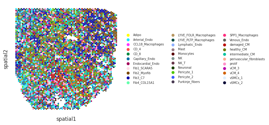
We can visualize cell type deconvolution results in slices (spots are colored by the the cell type with highest proportion). For this we will need the spatial coordinates of the spots in the Visium slices need to be in the slot uns[‘spatial’] of the Visium anndata object:
[11]:
mudata['visium'].uns['spatial']=mudata['visium'].obsm['X_spatial']
[12]:
idPat = 'GT_IZ_P9'
nichesphere.coloc.spatialCTPlot(adata=mudata['visium'][mudata['visium'].obs.patient_region_id==idPat].copy(),
                                CTprobs=CTprops.loc[spotSamples.index[spotSamples==idPat]],
                                cell_types=mudata['sc'].obs.cell_subtype2, spot_size=0.015,
                                legend_fontsize=7)
WARNING: saving figure to file figures/showtest.pdf
[ ]:
3.1 During differential co-localization analysis
We will compute then co-localization probabilities from the cell type probability matrices. Here will get concatenated co-localization sample matrices of cell type x cell type.
[13]:
CTcolocalizationP=nichesphere.coloc.getColocProbs(CTprobs=CTprops,
                                                  spotSamples=mudata['visium'].obs.patient_region_id #Series of spot samples with spot ID as index
                                                 )
Then we reshape the co-localization data into a matrix of cell type pairs x samples. We set the parameter complete = 1 because we have a simetrical matrix including both co-localization probabilities of cell type pair a - b , as well as b - a (which have the same probability)
[14]:
colocPerSample=nichesphere.coloc.reshapeColoc(CTcoloc=CTcolocalizationP,
                                              complete=1)
colocPerSample.head()
[14]:
| Fib1_SCARA5-Fib1_SCARA5 | Fib1_SCARA5-damaged_CM | Fib1_SCARA5-Capillary_Endo | Fib1_SCARA5-LYVE_FOLR_Macrophages | Fib1_SCARA5-Fib3_C7 | Fib1_SCARA5-healthy_CM | Fib1_SCARA5-Fib2_Myofib | Fib1_SCARA5-Endocardial_Endo | Fib1_SCARA5-Arterial_Endo | Fib1_SCARA5-Neuronal | ... | NK_T-CCL18_Macrophages | NK_T-perivascular_fibroblasts | NK_T-CD_4 | NK_T-vSMCs_2 | NK_T-Lymphatic_Endo | NK_T-NK | NK_T-CD_8 | NK_T-Purkinje_fibers | NK_T-Adipo | NK_T-NK_T | |
|---|---|---|---|---|---|---|---|---|---|---|---|---|---|---|---|---|---|---|---|---|---|
| control_P17 | 0.017603 | 0.000308 | 0.000992 | 0.000251 | 0.007062 | 0.002586 | 0.004724 | 0.000943 | 0.000412 | 0.000351 | ... | 2.290066e-15 | 0.0 | 3.915381e-05 | 0.0 | 0.0 | 4.538656e-08 | 4.556003e-08 | 0.0 | 0.000000e+00 | 0.000268 |
| RZ_P9 | 0.009307 | 0.000429 | 0.000738 | 0.000003 | 0.005204 | 0.001439 | 0.001625 | 0.000065 | 0.000168 | 0.000046 | ... | 0.000000e+00 | 0.0 | 4.640548e-05 | 0.0 | 0.0 | 9.954633e-05 | 1.643486e-05 | 0.0 | 0.000000e+00 | 0.000784 |
| IZ_P15 | 0.030351 | 0.000000 | 0.000027 | 0.000186 | 0.001200 | 0.000000 | 0.003112 | 0.000072 | 0.000062 | 0.000000 | ... | 0.000000e+00 | 0.0 | 0.000000e+00 | 0.0 | 0.0 | 0.000000e+00 | 0.000000e+00 | 0.0 | 0.000000e+00 | 0.000000 |
| RZ_P6 | 0.040470 | 0.000441 | 0.002752 | 0.000361 | 0.008687 | 0.002928 | 0.007878 | 0.000176 | 0.001022 | 0.001170 | ... | 0.000000e+00 | 0.0 | 7.998369e-25 | 0.0 | 0.0 | 8.593925e-28 | 0.000000e+00 | 0.0 | 0.000000e+00 | 0.000438 |
| RZ_BZ_P3 | 0.021508 | 0.000292 | 0.000567 | 0.000057 | 0.002408 | 0.000483 | 0.006635 | 0.000123 | 0.000052 | 0.000052 | ... | 0.000000e+00 | 0.0 | 0.000000e+00 | 0.0 | 0.0 | 8.585311e-06 | 0.000000e+00 | 0.0 | 7.294563e-35 | 0.000897 |
5 rows × 1089 columns
The sum of the probabilities of every cell type pair in a sample must be = 1
[15]:
colocPerSample.sum(axis=1)
[15]:
control_P17    1.0
RZ_P9          1.0
IZ_P15         1.0
RZ_P6          1.0
RZ_BZ_P3       1.0
FZ_P14         1.0
RZ_BZ_P12      1.0
FZ_GT_P4       1.0
GT_IZ_P13      1.0
GT_IZ_P15      1.0
FZ_P20         1.0
RZ_FZ_P5       1.0
GT_IZ_P9       1.0
RZ_P3          1.0
FZ_GT_P19      1.0
FZ_P18         1.0
IZ_P10         1.0
control_P7     1.0
RZ_P11         1.0
control_P1     1.0
RZ_BZ_P2       1.0
control_P8     1.0
RZ_GT_P2       1.0
dtype: float64
This is how we got the file from zenodo colocPerSample.csv
[16]:
colocPerSample=pd.read_csv('colocPerSample.csv', index_col=0)
colocPerSample.head()
[16]:
| Fib1_SCARA5-Fib1_SCARA5 | Fib1_SCARA5-damaged_CM | Fib1_SCARA5-Capillary_Endo | Fib1_SCARA5-LYVE_FOLR_Macrophages | Fib1_SCARA5-Fib3_C7 | Fib1_SCARA5-healthy_CM | Fib1_SCARA5-Fib2_Myofib | Fib1_SCARA5-Endocardial_Endo | Fib1_SCARA5-Arterial_Endo | Fib1_SCARA5-Neuronal | ... | NK_T-CCL18_Macrophages | NK_T-perivascular_fibroblasts | NK_T-CD_4 | NK_T-vSMCs_2 | NK_T-Lymphatic_Endo | NK_T-NK | NK_T-CD_8 | NK_T-Purkinje_fibers | NK_T-Adipo | NK_T-NK_T | |
|---|---|---|---|---|---|---|---|---|---|---|---|---|---|---|---|---|---|---|---|---|---|
| control_P17 | 0.017603 | 0.000308 | 0.000992 | 0.000251 | 0.007062 | 0.002586 | 0.004724 | 0.000943 | 0.000412 | 0.000351 | ... | 2.290066e-15 | 0.0 | 3.915381e-05 | 0.0 | 0.0 | 4.538656e-08 | 4.556003e-08 | 0.0 | 0.000000e+00 | 0.000268 |
| RZ_P9 | 0.009307 | 0.000429 | 0.000738 | 0.000003 | 0.005204 | 0.001439 | 0.001625 | 0.000065 | 0.000168 | 0.000046 | ... | 0.000000e+00 | 0.0 | 4.640548e-05 | 0.0 | 0.0 | 9.954633e-05 | 1.643486e-05 | 0.0 | 0.000000e+00 | 0.000784 |
| IZ_P15 | 0.030351 | 0.000000 | 0.000027 | 0.000186 | 0.001200 | 0.000000 | 0.003112 | 0.000072 | 0.000062 | 0.000000 | ... | 0.000000e+00 | 0.0 | 0.000000e+00 | 0.0 | 0.0 | 0.000000e+00 | 0.000000e+00 | 0.0 | 0.000000e+00 | 0.000000 |
| RZ_P6 | 0.040470 | 0.000441 | 0.002752 | 0.000361 | 0.008687 | 0.002928 | 0.007878 | 0.000176 | 0.001022 | 0.001170 | ... | 0.000000e+00 | 0.0 | 7.998369e-25 | 0.0 | 0.0 | 8.593925e-28 | 0.000000e+00 | 0.0 | 0.000000e+00 | 0.000438 |
| RZ_BZ_P3 | 0.021508 | 0.000292 | 0.000567 | 0.000057 | 0.002408 | 0.000483 | 0.006635 | 0.000123 | 0.000052 | 0.000052 | ... | 0.000000e+00 | 0.0 | 0.000000e+00 | 0.0 | 0.0 | 8.585311e-06 | 0.000000e+00 | 0.0 | 7.294563e-35 | 0.000897 |
5 rows × 1089 columns
The sum of the probabilities of every cell type pair in a sample must be = 1
[17]:
colocPerSample.sum(axis=1)
[17]:
control_P17    1.0
RZ_P9          1.0
IZ_P15         1.0
RZ_P6          1.0
RZ_BZ_P3       1.0
FZ_P14         1.0
RZ_BZ_P12      1.0
FZ_GT_P4       1.0
GT_IZ_P13      1.0
GT_IZ_P15      1.0
FZ_P20         1.0
RZ_FZ_P5       1.0
GT_IZ_P9       1.0
RZ_P3          1.0
FZ_GT_P19      1.0
FZ_P18         1.0
IZ_P10         1.0
control_P7     1.0
RZ_P11         1.0
control_P1     1.0
RZ_BZ_P2       1.0
control_P8     1.0
RZ_GT_P2       1.0
dtype: float64
Conditions
In this case, condition can be inferred from abbreviations in the sample names:
RZ = Remote zone BZ = Border Zone FZ = Fibrotic Zone IZ = Ischemic Zone
[18]:
sampleTypesDF=pd.DataFrame(colocPerSample.index, columns=['sample'])
sampleTypesDF['sampleType']='myogenic'

#tmp.obs.sampleType[tmp.obs['sample'].str.contains("BZ")]='border'
sampleTypesDF.sampleType[sampleTypesDF['sample'].str.contains("RZ")]='remote'
sampleTypesDF.sampleType[sampleTypesDF['sample'].str.contains("BZ")]='border'


sampleTypesDF.sampleType[sampleTypesDF['sample'].str.contains("FZ")]='fibrotic'
sampleTypesDF.sampleType[sampleTypesDF['sample'].str.contains("IZ")]='ischemic'
sampleTypesDF
[18]:
| sample | sampleType | |
|---|---|---|
| 0 | control_P17 | myogenic |
| 1 | RZ_P9 | remote |
| 2 | IZ_P15 | ischemic |
| 3 | RZ_P6 | remote |
| 4 | RZ_BZ_P3 | border |
| 5 | FZ_P14 | fibrotic |
| 6 | RZ_BZ_P12 | border |
| 7 | FZ_GT_P4 | fibrotic |
| 8 | GT_IZ_P13 | ischemic |
| 9 | GT_IZ_P15 | ischemic |
| 10 | FZ_P20 | fibrotic |
| 11 | RZ_FZ_P5 | fibrotic |
| 12 | GT_IZ_P9 | ischemic |
| 13 | RZ_P3 | remote |
| 14 | FZ_GT_P19 | fibrotic |
| 15 | FZ_P18 | fibrotic |
| 16 | IZ_P10 | ischemic |
| 17 | control_P7 | myogenic |
| 18 | RZ_P11 | remote |
| 19 | control_P1 | myogenic |
| 20 | RZ_BZ_P2 | border |
| 21 | control_P8 | myogenic |
| 22 | RZ_GT_P2 | remote |
This is how we got the file in zenodo MI_sampleTypesDF.csv
4. For differential communication
NicheSphere is suited to work with CrossTalkeR output tables which contain columns called cellpair, indicating the cell types involved in an interaction separated by ‘@’; and allpair, indicating cell types, ligand and receptor involved. Additionally, input tables for NicheSphere should contain columns indicating the ligand (gene_A), receptor (gene_B) and communication score (MeanLR). The names for these last 3 columns can be indicated in NicheSphere functions.
The following tables come from a CrossTalkeR run comparing myogenic and ischemic samples. They are the condition specific tables in the LR_data_final object:
[19]:
crossTalker_ctrlComm=pd.read_csv('./crossTalker_tbl_myo_heart_exp_scSeqComm.csv', index_col=0)
crossTalker_iscComm=pd.read_csv('./crossTalker_tbl_isc_heart_exp_scSeqComm.csv', index_col=0)
CrossTalkeR tables contain strings indicating wether a gene is a ligand (|L), receptor (|R) or transcription factor (|TF). These strings will be removed as they might cause conflicts with code.
[20]:
crossTalker_ctrlComm=nichesphere.tl.processCTKRoutput(crossTalker_ctrlComm)
crossTalker_iscComm=nichesphere.tl.processCTKRoutput(crossTalker_iscComm)
4.1 Database
We are interested in cell communication related to fibrosis, so we will use a database which classifies ligands according to extracellular matrix (ECM) or immune cell recruitment related processes to look for disease related processes :
[21]:
allDBs=pd.read_csv('nichesphereDB_pmid.csv', index_col=0)
allDBs.head()
[21]:
| Ligand | category | db | PMID | |
|---|---|---|---|---|
| 2 | col1a1 | Collagens | matrisome | 36399478 |
| 3 | col1a2 | Collagens | matrisome | 36399478 |
| 4 | col1a1 | Collagens | matrisome | 36399478 |
| 5 | col6a3 | Collagens | matrisome | 36399478 |
| 6 | col1a2 | Collagens | matrisome | 36399478 |
[22]:
sns.barplot(x=allDBs.category.value_counts(), y=allDBs.category.value_counts().index,
            data=pd.DataFrame(allDBs.category.value_counts()))
[22]:
<Axes: xlabel='count', ylabel='category'>

4.2 During differential communication analysis
Now we can separate communication scores by process to know which cell type pairs and niche pairs are interacting through which processes in each condition.
Same cell type interactions will be excluded, so we’ll have a list of same cell type interaction pairs in order to subset the data.
[23]:
cell_types=CTprops.columns
oneCTints=cell_types+'-'+cell_types
For the calculation of the LR scores per process we will need the cell pair - niche pair correspondence table generated in the co-localization tutorial as pairCatDFdir
[24]:
pairCatDFdir=pd.read_csv('./pairCatDFdir_MIvisium_louvain.csv')
[25]:
myoCTpairScores_byCat2_dir_colocClusts=nichesphere.comm.lr_ctPairScores_perCat_dir(ccommTable=crossTalker_ctrlComm,
                                                                                   db=allDBs, dbCatCol='category',
                                                                                   dbMatchCol='Ligand',        #column in database table to match with (ligand) column in the communication data table
                                                                                   ccommMatchCol='gene_A',     #column in communication data table to match with (ligand) column in the database table
                                                                                   ccommLRscoresCol='MeanLR',
                                                                                   oneCTinteractions=oneCTints.str.replace('-', '@'),
                                                                                   condition='myogenic',
                                                                                   pairCatDF=pairCatDFdir)
[27]:
iscCTpairScores_byCat2_dir_colocClusts=nichesphere.comm.lr_ctPairScores_perCat_dir(ccommTable=crossTalker_iscComm,
                                                                                   db=allDBs,
                                                                                   dbCatCol='category',
                                                                                   dbMatchCol='Ligand',
                                                                                   ccommMatchCol='gene_A',
                                                                                   ccommLRscoresCol='MeanLR',
                                                                                   oneCTinteractions=oneCTints.str.replace('-', '@'),
                                                                                   condition='ischemic',
                                                                                   pairCatDF=pairCatDFdir)
[28]:
myoCTpairScores_byCat2_dir_colocClusts.head()
[28]:
| Unnamed: 0 | cell_pairs | niche_pairs | LRscores | LRcat | condition | |
|---|---|---|---|---|---|---|
| allpair | ||||||
| Adipo/COL14A1@Arterial_Endo/CD44 | 1031 | Adipo->Arterial_Endo | 1_Stromal->3_Healthy_CM | 0.717175 | Collagens | myogenic |
| Adipo/COL14A1@CCL18_Macrophages/CD44 | 1046 | Adipo->CCL18_Macrophages | 1_Stromal->4_Fibrotic | 0.967985 | Collagens | myogenic |
| Adipo/COL14A1@CD_4/CD44 | 1048 | Adipo->CD_4 | 1_Stromal->2_Stressed_CM | 0.967985 | Collagens | myogenic |
| Adipo/COL14A1@CD_8/CD44 | 1052 | Adipo->CD_8 | 1_Stromal->2_Stressed_CM | 0.967985 | Collagens | myogenic |
| Adipo/COL14A1@Fib1_SCARA5/CD44 | 1023 | Adipo->Fib1_SCARA5 | 1_Stromal->1_Stromal | 0.967985 | Collagens | myogenic |
Some interactions might be present only in one condition, so we will assign 0 values to the interactions that do not appear in one condition to be able to compare conditions
[31]:
myoCTpairScores_byCat2_dir_colocClusts, iscCTpairScores_byCat2_dir_colocClusts = nichesphere.comm.equalizeScoresTables(ctrlTbl=myoCTpairScores_byCat2_dir_colocClusts,
                                                                                                                       expTbl=iscCTpairScores_byCat2_dir_colocClusts,
                                                                                                                       ctrlCondition='myogenic',
                                                                                                                       expCondition='ischemic')
[32]:
myoCTpairScores_byCat2_dir_colocClusts.head()
[32]:
| Unnamed: 0 | cell_pairs | niche_pairs | LRscores | LRcat | condition | |
|---|---|---|---|---|---|---|
| allpair | ||||||
| Adipo/COL14A1@Arterial_Endo/CD44 | 1031 | Adipo->Arterial_Endo | 1_Stromal->3_Healthy_CM | 0.717175 | Collagens | myogenic |
| Adipo/COL14A1@CCL18_Macrophages/CD44 | 1046 | Adipo->CCL18_Macrophages | 1_Stromal->4_Fibrotic | 0.967985 | Collagens | myogenic |
| Adipo/COL14A1@CD_4/CD44 | 1048 | Adipo->CD_4 | 1_Stromal->2_Stressed_CM | 0.967985 | Collagens | myogenic |
| Adipo/COL14A1@CD_8/CD44 | 1052 | Adipo->CD_8 | 1_Stromal->2_Stressed_CM | 0.967985 | Collagens | myogenic |
| Adipo/COL14A1@Fib1_SCARA5/CD44 | 1023 | Adipo->Fib1_SCARA5 | 1_Stromal->1_Stromal | 0.967985 | Collagens | myogenic |
And this is how we get the tables processed_myo_ctkr_louvainColoc.csv and processed_isc_ctkr_louvainColoc.csv from zenodo
[ ]: